Shot noise is fluctuation associated with discrete transfer events. For an electric current, individual charge carriers contribute finite amounts of electric charge, even when a meter displays a smooth mean. The simplest model is a stream of equal, independently arriving charges with constant rate: its Poisson process predicts both the mean electric current and the variance around it. Discreteness alone does not imply a Poisson distribution; the timing and correlations matter.
The useful surprise is that noise can reveal something a mean hides. Two devices can carry the same mean electric current yet have different fluctuations because one transfers charges independently and the other groups or regulates them. A calibrated shot noise photocurrent measurement can connect a macroscopic voltage variance to the elementary charge. Thermal electrical noise instead exists in an unbiased resistor at thermal equilibrium; a measured background can contain both mechanisms.
Walter Schottky's 1918 paper Über spontane Stromschwankungen in verschiedenen Elektrizitätsleitern treated amplifier sensitivity limits. Part II considered independent discrete transfers, including thermionic emission through a vacuum. On p. 563 he proposed amplifying fluctuations from a separate discharge tube to determine the elementary charge; those experiments were prospective, not reported results.[ref]
Über spontane Stromschwankungen in verschiedenen Elektrizitätsleitern by Walter Schottky. Schottky (1918), p. 541; Part II, pp. 547–552; p. 563, proposed experiment
Let be the magnitude of each transferred electric charge, and let arrivals form a Homogeneous Poisson process of rate . Extend the stream over past and future times when considering stationary filtering. For Electrons, , the elementary charge. Choose the positive electric current direction to follow these transfers, so is its mean magnitude. If counts arrivals in a gate of duration , thenThe gate's transferred electric charge is , and its average electric current is . Scaling the expected value and variance givesMore arrivals increase the absolute fluctuation but decrease its size relative to the mean. For an original count example with , the mean count and its variance are both , the standard deviation is , and the relative standard deviation is . The probability of no transfer is ; the probability of four is . A constant arrival rate does not prescribe four arrivals in every gate.
These are fluctuations of a time average, not the variance of an ideal instantaneous electric current. A model of point transfers has arbitrarily sharp impulses; it acquires a finite measured variance only after specifying a gate or linear filter. Actual collection pulses have finite duration and electrical circuits have finite response times.
Write an ideal point-transfer model using the Dirac delta function:For this arrival stream with independent increments, distinct arrivals contribute the product of the means, which cancels when centering. The same-arrival term leaves the autocovarianceIts Fourier transform gives the two-sided power spectral density, while folding negative frequencies onto positive ones gives the one-sided convention:These spectra describe , excluding the spectral line from the mean direct current. The amplitude spectral density is in ; it is not a root mean square electric current until a measurement signal bandwidth is specified. Approximate white noise requires frequencies low enough that the single-transfer pulse shape and any correlations can be neglected. Neither the ideal impulses nor a flat spectrum extending to infinity describe a real detector at every timescale.
All spectra above are per hertz, with in cycles per second. One possible angular frequency convention defines a density integrated using alone. Since , it hasAnother common convention keeps the numerical density but integrates it with . State the integration measure as well as whether a spectrum is one-sided: a change of variable and a folding of signs are separate operations.
Let be the complete current-to-voltage frequency response from detector input to readout, in . For a real stable linear time-invariant system, the shot contribution to the output voltage variance isIf with feedback electrical resistance , a reference voltage gain , and dimensionless normalized frequency response , thenThis is the effective noise bandwidth for unit reference magnitude. The transimpedance amplifier factor converts electric current to voltage; multiplies voltage. Neither is an additional noise source merely because it amplifies an existing fluctuation. In contrast, a real amplifier adds input voltage noise and input current noise, and its feedback resistor contributes thermal electrical noise. Those terms need their own transfers to the output. In particular, input voltage noise generally has a different transfer from an injected detector electric current. Simply multiplying every input specification by is incorrect.
For a unit-gain exponential low-pass filter, with time constant ,The cutoff frequency is not . An independent time-domain derivation sums independent event contributions to giveThe same reasoning for a rectangular averaging gate has on and zero elsewhere, hence effective noise bandwidth and variance , agreeing with the shot noise counting model. Equal numerical durations do not make these two different linear filters equivalent.
For an original model, set , , , , and the exponential low-pass filter's . Assume an ideal detector without charge multiplication and omit all additive noise for this calculation. ThenDoubling doubles the voltage variance and multiplies its standard deviation by . Halving also doubles the variance, provided the detector remains approximately white throughout the enlarged passband. Using in place of underestimates the variance by the factor . These are calculated predictions, not measured values or settings claimed for the laboratory below.
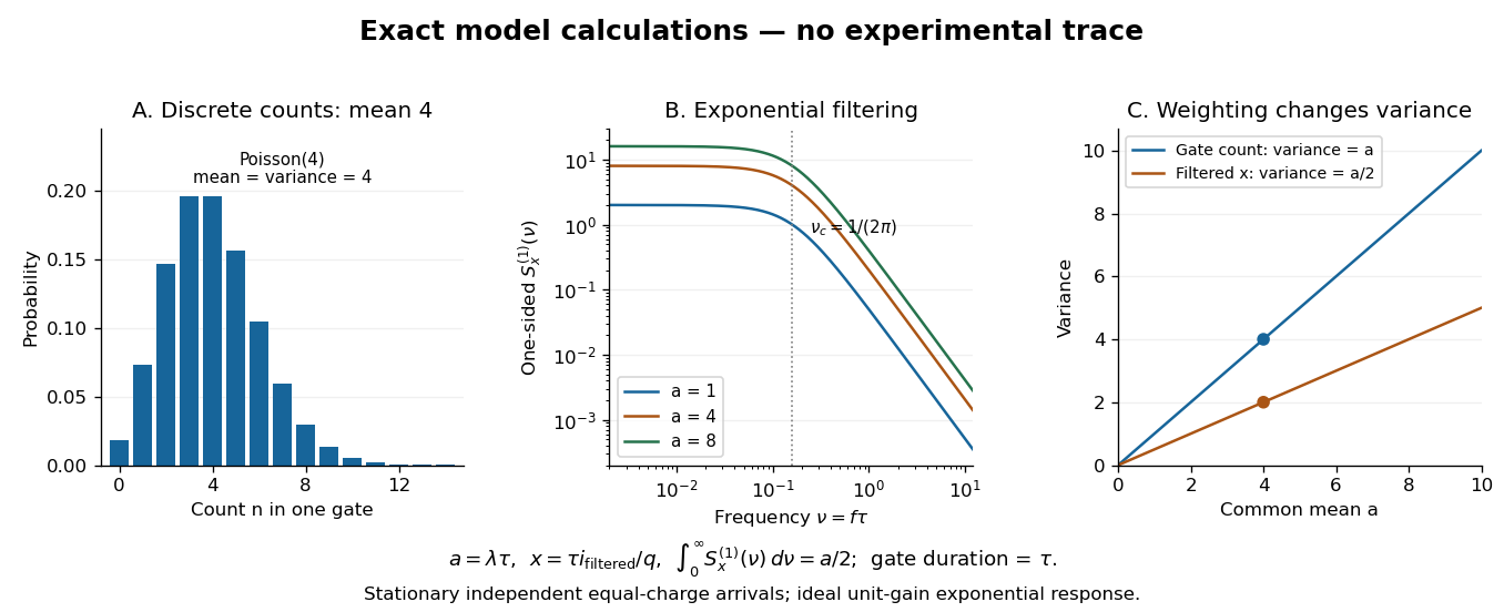
To read the dimensionless figure, set and , with frequency in cycles per unit . A gate of duration has count mean and variance . The continuously filtered instead hasThe count and the filtered electric current are different observables. The factor comes from the exponential weighting, not from non-Poisson arrivals. The dimensionless count illustration is a separate choice of rate; it does not assert that the example has only four Electrons per .
MIT's guide uses an illuminated vacuum photodiode, with collecting anode positive relative to the emitting cathode. A transimpedance amplifier gives ; a multimeter reads its mean. The fluctuation path rejects below , adds roughly tenfold voltage gain, then nominal hundredfold preamplification and a – band-pass filter; the readout measures root mean square voltage. With diode bias off, a sinusoid at the test port calibrates . Restore bias, retain gain settings, vary lamp brightness, and repeat both readings. The guide warns about overload; it supplies a procedure, not measured results.[ref]
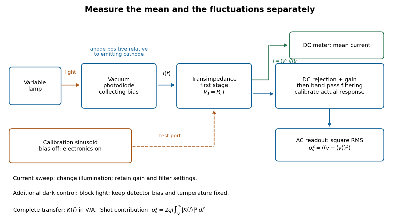
Functional photocurrent measurement: separate mean-current, fluctuation and calibration paths
. Original functional diagram organizing the laboratory's measurement roles; it is not a component-level circuit reproduction. includes current-to-voltage conversion and the complete fluctuation path. The dark comparison below is an additional control. Details.The inference can be expressed without relying on nominal passband edges. Let denote the calibrated voltage transfer after the conversion, so and define . Under independent arrivals and an unchanged additive background,The slope of voltage variance against mean electric current can therefore estimate . A free intercept accounts for a constant background; forcing the line through zero generally biases the slope. The root mean square readings must have their mean removed and then be squared. Subtracting two root mean square amplitudes does not subtract independent variances. Estimate the variance from successive records; averaging the waveforms first would suppress the fluctuation being measured.
Additional controls sharpen this interpretation. Block the light with detector bias, temperature, and gain unchanged; this preserves dark current and electronics while removing photocurrent. Repeat this dark comparison between illumination settings to check drift. If independent dark arrivals have mean magnitude and illuminated arrivals add , their spectra add: . Subtracting the unchanged dark variance isolates . This subtraction model assumes unchanged transfers and independence; switching off bias for gain calibration is a different control and need not preserve the dark background.
Vary measured rather than assuming lamp knob position is proportional to photocurrent. Check collection versus bias to identify a range where incomplete collection is negligible; a space charge limited tube can correlate transfers. Verify that the transimpedance amplifier remains linear and that its frequency response is unchanged over the illumination range. Changing signal bandwidth should change the excess variance through ; compare inferred input spectra in several bands. Correlated fluctuations of the light source can add a contribution scaling approximately as , while an electronics floor can hide the linear term at small electric currents. A fitted line over a short range alone does not establish independent transfers.
The gain calibration must include the same detector-to-readout path used for noise, or explicitly supply any omitted transfer. Detector capacitance, finite collection time, amplifier voltage and current noise, thermal electrical noise, pickup, clipping, and finite recording precision limit the inference. Current-dependent electrical impedance or heating can make a background current-dependent too. Since contains squared gain, a small fractional error in gain produces approximately twice that fractional error in the predicted variance scale. Knowing a nominal gain and two cutoff settings is insufficient.
The Fano factor compares count variance with its mean over a specified gate. For a stationary unidirectional stream with fixed charge , finite count second moments, and a generalized autocovariance with finite integral so that the long-gate limit exists,The zero-frequency relation concerns the continuous fluctuation spectrum, excluding the mean spectral line. It follows by writing as the double integral of the current autocovariance; for long , its leading term is . A finite-gate , a frequency-dependent ratio , and a factor inferred from one filtered variance are not interchangeable. The last is weighted by the instrument's .
Two original counting counterexamples show why electric charge discreteness is insufficient. In independent time slots, transfer one charge with probability in each slot: the binomial distribution gives mean , variance and Fano factor . A random common origin for the slots removes a preferred time origin; the long-gate factor remains . Alternatively, if independent Poisson process bursts each transfer exactly two charges, then gives and factor . Both count individual charges; only the first model allows at most one per slot, and the second groups them in pairs.
Consequently is a reference for independent unidirectional arrivals, not a universal noise law for all electrical conductors. Correlations, charge multiplication, and bidirectional transfer require a more specific model. For example, independent opposite streams with positive current magnitudes and have net mean but one-sided fluctuation spectrum . Using would miss their fluctuations when the net current is small. At thermal equilibrium, the full transport model must also respect thermal electrical noise; adding unrelated phenomenological formulas can double count the same underlying transfers.
Articles by others on the same topic



Shot noise is a type of electronic noise that arises from the discrete nature of charge carriers, such as electrons, in a system. It is particularly significant in situations where current is low, and it becomes more pronounced in semiconductor devices, photodetectors, and other electronic components that rely on the movement of individual charge carriers.