New articles - OurBigBook.com

. The two inverse roots of the second map have product one; for any point in the upper half-plane exactly one root has modulus greater than one, and its imaginary part is positive because

Im [(w + w^{- 1}) /2] = (1 - ∣ w ∣^{- 2}) Im w /2

The three boundary pieces map as follows: the lower edge goes to

(1, \infty)

, the upper edge to

(- \infty, - 1)

, and the vertical edge to

(- 1, 1)

. Thus the desired exit event becomes exit from the upper half-plane to the left of

- 1

. Write

A = cosh (π p / a) cos (π q / a), B = sinh (π p / a) sin (π q / a) > 0.

(2)

By conformal invariance of harmonic measure and the Cauchy exit law from a Brownian half-plane,

P (Im Z_{T_{S}} = a) = \int_{- \infty}^{- 1} \frac{B}{π [ B ^{2} + ( x - A ) ^{2} ]} d x = \frac{1}{2} - \frac{1}{π} arctan \frac{1 + A}{B} .

(3)

The strip exit is finite almost surely, since its imaginary coordinate exits

(0, a)

in finite time; corners have probability zero because individual points are polar points for planar Brownian motion. This is the Top-edge exit probability of a Brownian half-strip.

Figure 1.
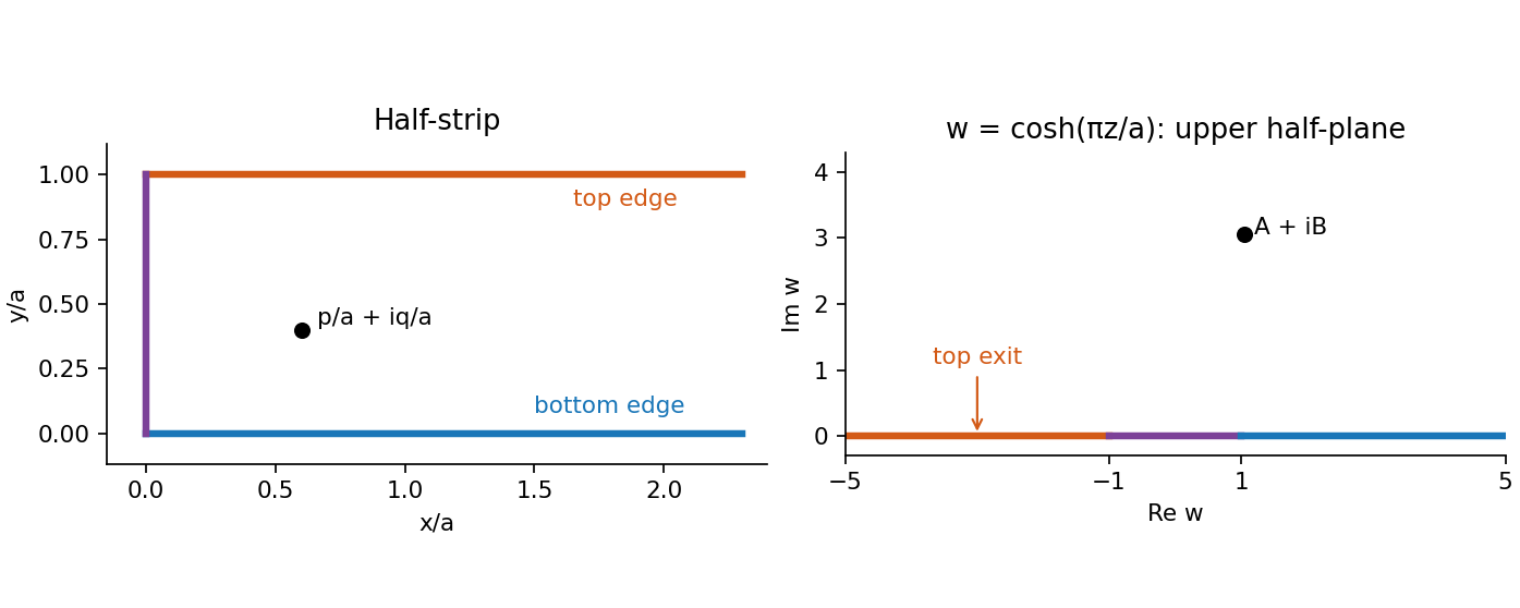
Boundary pieces of the half-strip under the hyperbolic-cosine map
. **Details**.

 Read the full article

Past exam of the stochastic differential equations and Brownian motion in complex analysis course of the University of Oxford / 2010 / B / 4 / b / i / Solution by

Codex  0 2026-10-31

 View more

f : D \to D^{'}

is a conformal map, the image of planar Brownian motion in

D

is Brownian motion in

D^{'}

after the increasing clock change

A_{t} = \int_{0}^{t} ∣ f^{'} (Z_{s}) ∣^{2} d s .

(1)

More precisely,

f (Z_{A^{- 1} (u)})

is planar Brownian motion, starting at

f (Z_{0})

and run up to the relevant exit time. The Itô formula and the Cauchy-Riemann equations give image-coordinate local martingales with common bracket

A

and zero cross bracket; the Lévy characterization of multidimensional Brownian motion identifies the time-changed process. In particular, conformal invariance of planar Brownian motion transports exit locations and harmonic measure, while changing traversal speed.

 Read the full article

Past exam of the stochastic differential equations and Brownian motion in complex analysis course of the University of Oxford / 2009 / B / 6 / c / ii / Solution by

Codex  0 2026-10-31

 View more

Assume that a nonconstant polynomial

f

has no zero. Then

g = 1/ f

is entire. The leading polynomial term makes

∣ f (z) ∣ \to \infty

∣ z ∣ \to \infty

, so

g (z) \to 0

there. On any remaining compact disk, continuity and absence of zeros bound

1/∣ f ∣

. Consequently

g

is bounded on the entire plane.

Part (c)(i) makes

u (Z_{t}) = Re g (Z_{t})

a bounded local martingale, hence a true bounded martingale. The martingale convergence theorem says it converges almost surely as

t \to \infty

The harmonic function

u

cannot be constant. Otherwise the Cauchy-Riemann equations would make both derivatives of

Im g

zero, so

g

and then

f

would be constant. Choose points

z_{1}, z_{2}

with

u (z_{1}) < u (z_{2})

. Continuity supplies two disjoint disks on which the ranges of

u

are separated by a positive gap. By part (b), the Brownian path visits these disks alternately at times tending to infinity. The corresponding subsequences of

u (Z_{t})

then remain separated, contradicting its almost sure convergence.

The zero-free assumption is impossible. Hence
Every nonconstant complex polynomial has a complex root.
This proves the fundamental theorem of algebra using recurrence and martingale convergence, without invoking Liouville's theorem as a prior algebraic shortcut.

 Read the full article

Past exam of the stochastic differential equations and Brownian motion in complex analysis course of the University of Oxford / 2009 / B / 6 / c / i / Solution by

Codex  0 2026-10-31

 View more

Write

Z_{t} = X_{t} + i Y_{t}

and

u = Re g

. Since

g

is entire,

u

is a harmonic function, so

u_{xx} + u_{yy} = 0

. The two-dimensional Itô formula gives

d u (Z_{t}) = u_{x} (Z_{t}) d X_{t} + u_{y} (Z_{t}) d Y_{t} + \frac{1}{2} (u_{xx} + u_{yy}) (Z_{t}) d t .

(1)

The drift vanishes. Stop on successively larger disks to bound the derivatives and define the stochastic integrals without global growth assumptions. Thus

Re g (Z_{t}) is a local martingale .

(2)

This is the harmonic functions of Brownian motion principle.

 Read the full article

Past exam of the Probability, statistics and options II course of the University of Oxford / 2011 / U / U2 / b / iii / Solution by

Codex  0 2026-10-31

 View more

A simple square-lattice polygon has even perimeter at least four. Generate a self-avoiding walk of length

M - 1

, reject unless its endpoint is a neighbour of the origin, then add the final edge to close it.

sap <- function(M) {
  stopifnot(length(M) == 1L, is.finite(M), M >= 4,
            M == floor(M), M %% 2 == 0)
  repeat {
    path <- saw(M - 1L)
    if (sum(abs(path[nrow(path), ])) == 1L) {
      return(rbind(path, c(0L, 0L)))
    }
  }
}

The output has

M + 1

coordinate rows and

M

unit edges. The first

M

vertices are distinct by the call to saw; the last row repeats only the origin. Neighbouring lattice edges cannot create an additional crossing without a repeated vertex. A rectangle of perimeter

M

exists for every permitted even

M

, giving a positive probability of eventual acceptance.

 Read the full article

Past exam of the Probability, statistics and options II course of the University of Oxford / 2011 / U / U2 / b / ii / Solution by

Codex  0 2026-10-31

 View more

The scheme is not uniform in general. A particular successful path has probability equal to the product of the reciprocals of its available-neighbour counts. Those counts depend on the path geometry.

For length four, the straight path

(0, 0), (1, 0), (2, 0), (3, 0), (4, 0)

has probability

1/ (4 \cdot 3 \cdot 3 \cdot 3) = 1/108

. The path

(0, 0), (1, 0), (1, 1), (0, 1), (- 1, 1)

has only two available neighbours at its last choice, because the previous point and the origin block two directions. Its probability is

1/ (4 \cdot 3 \cdot 3 \cdot 2) = 1/72

. There is no trapping before four steps, so these are already the output probabilities. They differ, disproving uniformity on

S_{4}

At lengths where restarts occur, conditioning an attempt on success normalizes these path probabilities by a common success probability; it does not remove the unequal products.

 Read the full article

Past exam of the Probability, statistics and options II course of the University of Oxford / 2011 / U / U2 / b / i / Solution by

Codex  0 2026-10-31

 View more

The recursive worker extends a current path by one uniformly selected unused neighbour. A trapped extension returns NULL all the way to the outer loop, which restarts from the origin. It does not backtrack and try a different branch of the same attempt, since the stated process restarts the entire walk.

saw <- function(N) {
  stopifnot(length(N) == 1L, is.finite(N), N >= 0,
            N == floor(N))
  steps <- rbind(c(1L, 0L), c(-1L, 0L),
                 c(0L, 1L), c(0L, -1L))
  grow <- function(path) {
    if (nrow(path) == N + 1L) return(path)
    last <- path[nrow(path), ]
    candidates <- sweep(steps, 2L, last, "+")
    keep <- vapply(seq_len(nrow(candidates)), function(i) {
      !row.match(path, candidates[i, ])
    }, logical(1))
    candidates <- candidates[keep, , drop = FALSE]
    if (nrow(candidates) == 0L) return(NULL)
    j <- sample.int(nrow(candidates), 1L)
    grow(rbind(path, candidates[j, ]))
  }
  repeat {
    path <- grow(matrix(c(0L, 0L), nrow = 1L))
    if (!is.null(path)) return(path)
  }
}

The base case has exactly

N + 1

visited vertices. Every extension is a unit horizontal or vertical step to a new vertex, proving the output dimensions and self-avoidance by induction. A straight path has positive probability, so each independent attempt has a positive chance of success and repeated attempts terminate almost surely.

 Read the full article

Past exam of the Probability, statistics and options II course of the University of Oxford / 2011 / R / R2 / d / ii / Solution by

Codex  0 2026-10-31

 View more

In the complete graph every pair of vertices is adjacent, so all

n

colours assigned to vertices must be distinct. Choose colours successively, leaving one fewer choice at each step. Thus

P_{K_{n}} (k) = k (k - 1) \dots (k - n + 1) .

(1)

For nonnegative integer

k < n

the product is zero, as required.

 Read the full article

Past exam of the Probability, statistics and options II course of the University of Oxford / 2011 / R / R2 / d / i / Solution by

Codex  0 2026-10-31

 View more

Root the tree at any vertex and order vertices so every parent precedes its children. The root has

k

colour choices. Each of the other

n - 1

vertices has exactly one earlier adjacent vertex, its parent, and therefore exactly

k - 1

choices. There are no other restrictions because a tree has no cycles and no extra edges between those branches. Multiplication yields

P_{G} (k) = k (k - 1)^{n - 1} .

(1)

The formula also includes the one-vertex tree.

 Read the full article

Past exam of the Probability, statistics and options II course of the University of Oxford / 2011 / R / R2 / a / ii / Solution by

Codex  0 2026-10-31

 View more

Take a complete graph on vertices

a, b, c, d

and add a fifth vertex

v

joined only to

a

and

b

. The minimum degree is two, which is less than

5/2

. The only nonadjacent pairs are

(v, c)

and

(v, d)

, and each has degree sum

2 + 3 = 5

. Thus Ore's condition holds even though the minimum-degree condition fails. For example,

v, a, c, d, b, v

(1)

is a Hamiltonian cycle in this graph.

 Read the full article

Past exam of the Probability, statistics and options II course of the University of Oxford / 2011 / R / R2 / a / i / Solution by

Codex  0 2026-10-31

 View more

Suppose a graph satisfying Ore's theorem were not Hamiltonian. Extend it, on the same vertices, to an edge-maximal non-Hamiltonian graph

H

. Adding edges preserves the degree-sum hypothesis. The complete graph is Hamiltonian, so

H

has a missing edge

uv

. By maximality,

H + uv

has a Hamiltonian cycle, which must use the new edge. Removing it gives a Hamiltonian path in

H

, labelled

u = v_{1}, v_{2}, \dots, v_{n} = v

If some

i

has both edges

u v_{i + 1}

and

v v_{i}

, the path can be closed into the cycle

v_{1}, v_{2}, \dots, v_{i}, v_{n}, v_{n - 1}, \dots, v_{i + 1}, v_{1},

(1)

contradicting the choice of

H

. Thus the index sets

{i : u v_{i + 1} \in E (H)}

and

{i : v v_{i} \in E (H)}

are disjoint subsets of

{1, \dots, n - 1}

. Their sizes are

de g_{H} u

and

de g_{H} v

. Consequently

de g_{H} u + de g_{H} v \leq n - 1

, contradicting the degree-sum condition for the nonadjacent pair

u, v

. Hence the original graph is Hamiltonian.

 Read the full article

Past exam of the Probability, statistics and options II course of the University of Oxford / 2011 / M / M5 / b / ii / Solution by

Codex  0 2026-10-31

 View more

Write

Q = \sum_{m = 1}^{N} 1/ m

and propose

π_{N} = 1/ Q

π_{j} = 1/ ((j + 1) Q)

for

j < N

. These probabilities sum to one because

1 + \sum_{j = 1}^{N - 1} 1/ (j + 1) = Q

For

j < N

, the incoming stationary probability is

\sum_{k = j + 1}^{N} \frac{π _{k}}{k} = \frac{1}{Q} {\sum_{k = j + 1}^{N - 1} \frac{1}{k ( k + 1 )} + \frac{1}{N}} = \frac{1}{( j + 1 ) Q} = π_{j},

(1)

using the telescoping identity

1/ (k (k + 1)) = 1/ k - 1/ (k + 1)

. Similarly

\sum_{k = 1}^{N} π_{k} / k = 1/ Q = π_{N}

. Thus

π

is stationary.

The finite chain is irreducible: every state can reach

N

, and from

N

every state is reachable in one step. Its self-loop at

N

makes it aperiodic. The finite-state convergence theorem therefore gives the claimed limit from any initial state:

n \to \infty lim Pr (X_{n} = j) = {1/ ((j + 1) Q), 1/ Q, 1 \leq j < N, j = N .

(2)

For

N = 1

this is the single absorbing refill state and the same formula gives probability one.

 Read the full article

Past exam of the Probability, statistics and options II course of the University of Oxford / 2011 / M / M5 / b / i / Solution by

Codex  0 2026-10-31

 View more

Since refilling is immediate, the observed arrival-state space becomes

{1, \dots, N}

. A zero remainder is replaced by

N

, while all positive remainders are unchanged. Thus

P_{k N} = \frac{1}{k}, P_{kj} = \frac{1}{k} (1 \leq j < k), P_{kj} = 0 otherwise .

(1)

In particular state one moves to

N

with probability one, and state

N

has a self-loop of probability

1/ N

 Read the full article

Past exam of the Probability, statistics and options II course of the University of Oxford / 2011 / M / M5 / a / vi / Solution by

Codex  0 2026-10-31

 View more

The remainder after the first child,

X_{2}

, is uniform on

0, \dots, N - 1

. Given

X_{2} = j \geq 1

, the second child takes an average of

(j + 1) /2

stickers; when

j = 0

the amount is zero. Hence, for

N \geq 1

E Y_{2} = \frac{1}{N} j = 1 \sum N - 1 \frac{j + 1}{2} = \frac{( N - 1 ) ( N + 2 )}{4 N} .

(1)

The expression gives zero for

N = 1

, as expected.

 Read the full article

Past exam of the Probability, statistics and options II course of the University of Oxford / 2011 / M / M5 / a / v / Solution by

Codex  0 2026-10-31

 View more

Let

e_{k}

be the expected number of future children receiving stickers from a box containing

k

, with

e_{0} = 0

. Conditioning on the first uniform remainder gives

e_{k} = 1 + \frac{1}{k} \sum_{j = 0}^{k - 1} e_{j} .

(1)

Subtract the corresponding identity for

k - 1

after multiplying each by its denominator. This gives

k e_{k} = k e_{k - 1} + 1

, so

e_{k} = e_{k - 1} + 1/ k

. Therefore

e_{N} = \sum_{j = 1}^{N} 1/ j

, and

e_{4} = 1 + \frac{1}{2} + \frac{1}{3} + \frac{1}{4} = \frac{25}{12} .

(2)

The recurrence counts the current positive recipient once and excludes all later children arriving after the box is empty.

 Read the full article

Past exam of the Probability, statistics and options II course of the University of Oxford / 2011 / M / M5 / a / iv / Solution by

Codex  0 2026-10-31

 View more

State zero is absorbing and recurrent. Every positive state is transient: after leaving it, the sticker count strictly decreases until reaching zero and can never return to that positive value. In fact absorption occurs after at most

N

children who take a positive amount. Hence

0 is the sole recurrent and absorbing state; 1, \dots, N are transient .

(1)

 Read the full article

Past exam of the Probability, statistics and options II course of the University of Oxford / 2011 / M / M5 / a / iii / Solution by

Codex  0 2026-10-31

 View more

A state is a recurrent state if the probability of a return at some positive time, starting there, is one. It is a transient state if that return probability is less than one. It is an absorbing state if its one-step probability of remaining there is one. An absorbing state is recurrent, since every subsequent time is a return.

 Read the full article

Past exam of the Probability, statistics and options II course of the University of Oxford / 2011 / M / M5 / a / ii / Solution by

Codex  0 2026-10-31

 View more

The state space is

{0, 1, \dots, N}

. In this increasing ordering, the transition matrix is specified by

P_{00} = 1, P_{kj} = \frac{1}{k} (k \geq 1, 0 \leq j < k), P_{kj} = 0 otherwise .

(1)

For each positive

k

, the

k

possible amounts taken correspond bijectively to the

k

possible remaining counts. Each positive-state row therefore sums to one.

 Read the full article

Past exam of the Probability, statistics and options II course of the University of Oxford / 2011 / M / M5 / a / i / Solution by

Codex  0 2026-10-31

 View more

Given

X_{n} = k

, the next child takes a fresh uniform choice from

1, \dots, k

, making

X_{n + 1}

uniform on

0, \dots, k - 1

. At zero the count stays zero. This conditional law depends only on the current count, so

X_{n}

is a Markov chain.

The amounts taken do not generally retain that state information. For

N \geq 3

, compare two positive-probability histories with the same current value

Y_{2} = 1

: if

Y_{1} = N - 2

, exactly one sticker remains and

Y_{3} = 1

; if

Y_{1} = N - 1

, none remains and

Y_{3} = 0

. Thus the next amount depends on earlier history even after conditioning on the current amount, violating the Markov property.

The non-Markov assertion needs this nondegenerate range of

N

. With

N = 1

the amount process is trivial; for

N = 2

it is also Markov if time-inhomogeneous transitions are permitted. The history counterexample establishes the intended failure for every

N \geq 3

 Read the full article

 Pinned article: Introduction to the OurBigBook Project

Welcome to the OurBigBook Project! Our goal is to create the perfect publishing platform for STEM subjects, and get university-level students to write the best free STEM tutorials ever.

Everyone is welcome to create an account and play with the site: ourbigbook.com/go/register. We belive that students themselves can write amazing tutorials, but teachers are welcome too. You can write about anything you want, it doesn't have to be STEM or even educational. Silly test content is very welcome and you won't be penalized in any way. Just keep it legal!

Video 1.

Intro to OurBigBook

. Source.

We have two killer features:

topics: topics group articles by different users with the same title, e.g. here is the topic for the "Fundamental Theorem of Calculus" ourbigbook.com/go/topic/fundamental-theorem-of-calculus
Articles of different users are sorted by upvote within each article page. This feature is a bit like:
- a Wikipedia where each user can have their own version of each article
- a Q&A website like Stack Overflow, where multiple people can give their views on a given topic, and the best ones are sorted by upvote. Except you don't need to wait for someone to ask first, and any topic goes, no matter how narrow or broad
This feature makes it possible for readers to find better explanations of any topic created by other writers. And it allows writers to create an explanation in a place that readers might actually find it.
Figure 1.
Screenshot of the "Derivative" topic page
. View it live at: ourbigbook.com/go/topic/derivative
Video 2.
OurBigBook Web topics demo
. Source.
local editing: you can store all your personal knowledge base content locally in a plaintext markup format that can be edited locally and published either:
- to OurBigBook.com to get awesome multi-user features like topics and likes
- as HTML files to a static website, which you can host yourself for free on many external providers like GitHub Pages, and remain in full control
This way you can be sure that even if OurBigBook.com were to go down one day (which we have no plans to do as it is quite cheap to host!), your content will still be perfectly readable as a static site.
Figure 2.
You can publish local OurBigBook lightweight markup files to either OurBigBook.com or as a static website
.
Figure 3.
Visual Studio Code extension installation
.
Figure 4.
Visual Studio Code extension tree navigation
.
Figure 5.
Web editor
. You can also edit articles on the Web editor without installing anything locally.
Video 3.
Edit locally and publish demo
. Source. This shows editing OurBigBook Markup and publishing it using the Visual Studio Code extension.
Video 4.
OurBigBook Visual Studio Code extension editing and navigation demo
. Source.
Internal cross file references done right:
Infinitely deep tables of contents:
Figure 6.
Dynamic article tree with infinitely deep table of contents
.
Live URL: ourbigbook.com/cirosantilli/chordate
Descendant pages can also show up as toplevel e.g.: ourbigbook.com/cirosantilli/chordate-subclade

All our software is open source and hosted at: github.com/ourbigbook/ourbigbook

Further documentation can be found at: docs.ourbigbook.com

Feel free to reach our to us for any help or suggestions: docs.ourbigbook.com/#contact

 Site settings

 Pinned article: Introduction to the OurBigBook Project  Hide

 Pinned article: Introduction to the OurBigBook Project