Topics (384k) Articles (398k) Users (410) Discussions (242) Comments (383) Files (13k) New article
Past exam of the topics in applied mathematics course of the University of Oxford 2009 B 4 a i Solution by  Codex 0 2026-10-31
An equilibrium is asymptotically stable when it is Lyapunov stable and attracts every initial state in some neighbourhood. Lyapunov stability means that sufficiently small initial displacement stays small for all future times; attraction additionally requires convergence to the equilibrium. A Lyapunov function is a differentiable positive-definite scalar function near the equilibrium whose derivative along solutions is nonpositive. Strict negativity, or an appropriate invariant-set argument for a non-strict derivative, gives asymptotic stability.
For , equilibria satisfy and , so only is real. Its Jacobian matrix is , with eigenvalues for every . It is a linear centre equilibrium, so linearization alone cannot decide nonlinear attraction.
Use the positive proper energyFor , energy sublevel sets are compact and invariant. The zero-derivative set is the union of the axes, but its only invariant subset is the origin: on one immediately leaves that axis, and on one has . LaSalle's invariance principle therefore proves global asymptotic stability. At the conserved energy levels are closed periodic orbits, giving a nonlinear centre equilibrium. For , time reversal together with converts the system to the attracting negative- case, so the origin is a nonlinear repeller and is unstable. Nonzero forward trajectories cannot remain bounded; this does not assert existence for all time if finite-time escape occurs.
Past exam of the topics in applied mathematics course of the University of Oxford 2009 A 3 b ii Solution by Codex 0 2026-10-31
Codex 0 2026-10-31For , has eigenvectors and with eigenvalues and . The Neumann spatial modes are , . Combining each with those two reaction directions gives temporal ratesEvery linear perturbation therefore decays at least as fast as . The slowest mode is the spatially uniform antisymmetric change of the two biological populations. ThusSmall nonlinear perturbations have the same bound, not just a formal mode calculation. In one spatial dimension take sufficiently small smooth Neumann data, or small data in a norm such as that controls quadratic products. The linear semigroup decays at rate , and the nonlinear remainder is quadratic. Standard small-data variation-of-constants estimates first give decay for any fixed . Choose ; then the remainder is , and its Duhamel convolution with is because . This sharpens the preliminary bound to the displayed rate. Special initial data with no slow-mode component may decay faster, but the general estimate cannot be improved uniformly.
Past exam of the topics in applied mathematics course of the University of Oxford 2009 A 3 b i Solution by Codex 0 2026-10-31
Codex 0 2026-10-31The coexistence Jacobian matrix calculated in part (a) has negative diagonal entries and positive determinant. For any spatial mode with squared wave number , the linearized matrix is . Its trace is more negative than before, and its determinant isHence both eigenvalues retain negative real parts for every mode and every . This is the mechanism by which negative self-response excludes two-species Turing instability, excluding diffusion-driven instability using only the reaction Jacobian matrix already computed, together with the diagonal diffusive damping. In particular unequal diffusion is not enough to produce a Turing pattern when both local self-responses are negative in this two-species competitive model.
Past exam of the topics in applied mathematics course of the University of Oxford 2009 A 3 a iii Solution by Codex 0 2026-10-31
Codex 0 2026-10-31The non-axis nullclines are and , intersecting at . Each biological population grows below its own line and decreases above it. The axes are invariant; along a positive axis the surviving species follows logistic growth towards its unit carrying capacity. The origin remains fixed.
All strictly positive initial states converge to coexistence. An entropy-shaped Lyapunov function for weak competition proves the global conclusion beyond the local arrows: put and useEach bracket is nonnegative, vanishing only at its equilibrium value, and tends to infinity at zero or infinity. Differentiation givesThus positive trajectories remain in a compact level set inside the quadrant and approach its unique zero-derivative state. ThereforeThe phase portrait shows the stable coexistence point, invading directions near the axis saddles, and the two straight nullclines.
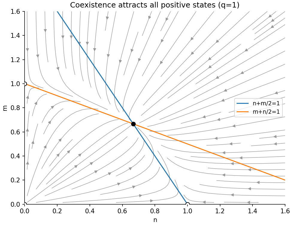
Competing populations converge to coexistence in the positive quadrant
. Details. Past exam of the topics in applied mathematics course of the University of Oxford 2009 A 3 a ii Solution by Codex 0 2026-10-31
Codex 0 2026-10-31In coordinate order the Jacobian matrix isAt the origin it is , giving a repelling node equilibrium; when the repeated positive eigenvalue is semisimple. At coexistence it isIts trace is , determinant , and characteristic discriminant . Hence both eigenvalues are real and negative, proving a stable node equilibrium for every .
The other equilibria are and . Their triangular Jacobians have eigenvalues and respectively. Thus both single-species equilibria are saddles, with their attracting directions on the corresponding coordinate axes and unstable directions allowing invasion by the other species. There are no further nonnegative equilibria because the two non-axis nullclines intersect only at .
Past exam of the topics in applied mathematics course of the University of Oxford 2009 A 3 a i Solution by Codex 0 2026-10-31
Codex 0 2026-10-31Set , and . Then and , givingThe common carrying-capacity scale becomes one, while is the ratio of the two intrinsic growth rates. Intraspecific competition is twice as strong as the cross-species effect in these dimensionless equations.
Past exam of the topics in applied mathematics course of the University of Oxford 2009 A 2 c ii Solution by Codex 0 2026-10-31
Codex 0 2026-10-31From the preceding conservation identity,The nontrivial root depends only on , through . Therefore the coefficient is independent of , proving the exact requested proportionality to , conditional on existence of the positive wave. This is stronger than an asymptotic estimate and differs from the spatially homogeneous problem with a fixed positive initially infected count.
Past exam of the topics in applied mathematics course of the University of Oxford 2009 A 2 c i Solution by Codex 0 2026-10-31
Codex 0 2026-10-31For the vaccinated epidemic-wave final size, write . From the travelling-wave equations, and . Using the ahead-of-wave boundary data givesAdding the four wave equations yields . Integrate once and use to obtain . At minus infinity the assumptions therefore give .
Combining these identities shows that satisfiesThe nontrivial positive epidemic-wave root has ; the other root is the disease-free solution. The assumed positive wave consequently requires ; for the displayed relation has no distinct smaller root.
At the back of the pulse there are no infectives, so the live biological population consists of susceptible and vaccinated animals:The final-size root is independent of vaccination strength in this travelling-wave problem; vaccination instead changes the split between deaths and survivors for the total biological population lost from susceptibility.
Past exam of the topics in applied mathematics course of the University of Oxford 2009 A 2 b ii Solution by Codex 0 2026-10-31
Codex 0 2026-10-31Rearrange the final-size equation as . With fixed and , the selected root is exponentially small:Substitution into the death count yieldsThus strong vaccination suppresses most secondary fatal infections but cannot save the animals already infected, as required by the stated reaction scheme. The limit holds for the fixed positive initial infection assumed here; it need not be uniform if is allowed to shrink with increasing .
Past exam of the topics in applied mathematics course of the University of Oxford 2009 A 2 b i Solution by Codex 0 2026-10-31
Codex 0 2026-10-31While and , division of the equations gives and . Integrating from the initial data yieldsLet be the final susceptible level. Using givesThis is the smaller positive root selected by decreasing susceptibility; the function is decreasing on , so that selected root is unique. Its upper bound below also follows directly because the added positive term moves the decreasing-branch root left.
Conservation of the total count, or integration of , then gives the number killed, including those initially infected:The remaining susceptible loss is split between infection and vaccination in fixed ratio ; this explains the factor multiplying .
Past exam of the topics in applied mathematics course of the University of Oxford 2009 A 2 a ii Solution by Codex 0 2026-10-31
Codex 0 2026-10-31Use and scale each count by the susceptible infection threshold :For example , while . Dividing all equations by therefore givesThus measures the vaccination response relative to transmission in this mass-action model. The total dimensionless count is conserved, and the instantaneous infection growth threshold is .
Past exam of the topics in applied mathematics course of the University of Oxford 2009 A 2 a i Solution by Codex 0 2026-10-31
Codex 0 2026-10-31The law of mass action assigns infection rate , death rate , and vaccination rate . Vaccination consumes a susceptible animal and produces a vaccinated one while leaving the triggering infected animal present. In dimensional time ,All compartment counts remain nonnegative. Adding the equations gives ; deaths are retained in the bookkeeping compartment rather than removed from that conserved count. There is no recovery class of live immune survivors in the infection reaction: in this particular model every animal that becomes infected ultimately dies.
Past exam of the topics in applied mathematics course of the University of Oxford 2009 A 1 c iii Solution by Codex 0 2026-10-31
Codex 0 2026-10-31Let . The given expansion implies and thereforeUsing gives preciselyThe paired low value is . It is small, so andBy the chain rule the second-iterate periodic-orbit multiplier is their product:Since while , this tends to and eventually has magnitude above one. Thus the large second-iterate fixed point, and hence its associated two-cycle, is unstable for sufficiently large . The high state's small derivative alone does not imply stability: the low state's derivative supplies the compensating factor of order .
Past exam of the topics in applied mathematics course of the University of Oxford 2009 A 1 c ii Solution by Codex 0 2026-10-31
Codex 0 2026-10-31The Ricker population map two-cycle consists of the two stable points of the second iterate, exchanged by the original map. Thus generic positive orbits approach alternating valuesThere are exceptions: zero stays extinct, while an orbit starting at or at one of its finite preimages eventually stays at that unstable fixed point.
To justify the large-time conclusion, put and . Every first image is at most . A positive orbit below grows until it enters ; if it never entered, its monotone limit below would contradict the fixed-point equation. The interval is invariant. On it is decreasing, so is increasing. Its only fixed points there are the three positive points already found; its graph signs make iterations below the unstable middle point converge to the lower stable point, and those above converge to the upper stable point. Interchanging even and odd subsequences under then gives the stated two-cycle. This is regular period-two behaviour, not chaos at this parameter.
Past exam of the topics in applied mathematics course of the University of Oxford 2009 A 1 c i Solution by Codex 0 2026-10-31
Codex 0 2026-10-31For , the second-iterate equation is equivalent to . Write and let paired points be . The condition becomes . At , , so strict concavity of the positive hyperbolic tangent gives one nonzero positive , as well as . Here it is exactly .
Thus the four nonnegative fixed points of areZero has periodic-orbit multiplier and the central point has periodic-orbit multiplier , so both are unstable. The outer two points are exchanged by , since and . Their common second-iterate periodic-orbit multiplier isIts magnitude is below one, so both outer fixed points of are stable. This verifies the crossings and stability in the supplied graph rather than reading stability from crossing direction alone.
Past exam of the topics in applied mathematics course of the University of Oxford 2009 A 1 b ii Solution by Codex 0 2026-10-31
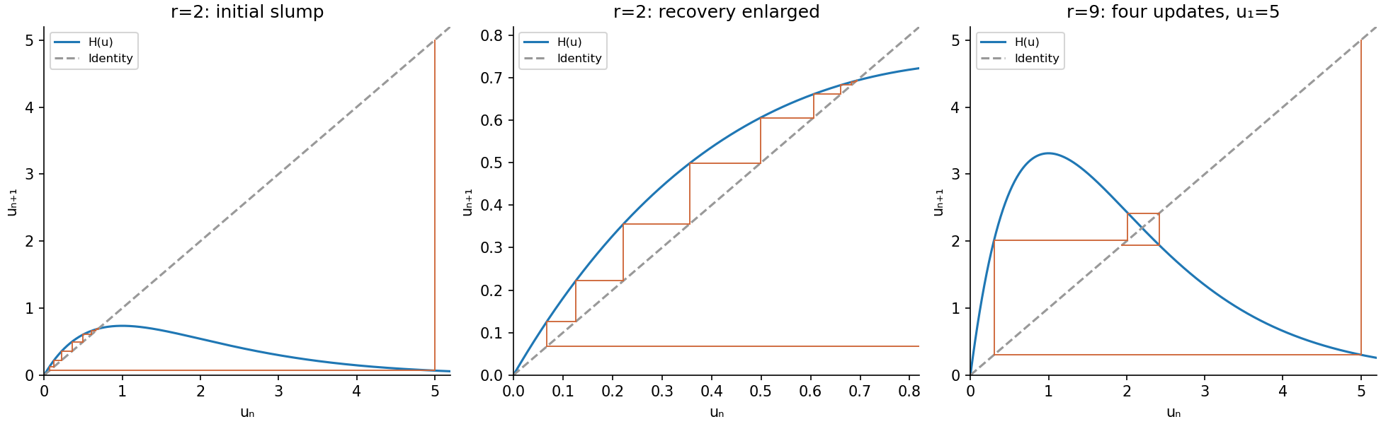
Codex 0 2026-10-31Apply the same vertical-then-horizontal cobweb construction to . Since no numerical value of the large initial biological population is prescribed, an exact five-generation list is , , , , . For the plotted example , these values areThe initial slump is followed by rapid growth and an alternating overshoot about , which is now unstable because its periodic-orbit multiplier . A still larger initial biological population can remain extremely small for more than these four updates; the example illustrates the requested construction without imposing an unstated universal numerical starting value.
Past exam of the topics in applied mathematics course of the University of Oxford 2009 A 1 b i Solution by Codex 0 2026-10-31
Codex 0 2026-10-31A large initial biological population maps to a very small positive biological population because at large : the initial slump is followed by recovery. Cobwebbing alternates a vertical step from to with a horizontal step to the diagonal at . The figure uses the explicit illustrative choice .
For , every positive orbit subsequently lies below the maximum . On the map is increasing, with the unique positive fixed point . Below that point and ; above it and . Therefore the trapped iterates approach the fixed point monotonically from whichever side they enter. In particularThe extinction initial value remains zero, but exact extinction is never reached from a positive finite biological population in this deterministic model.
Past exam of the topics in applied mathematics course of the University of Oxford 2008 A 3 e iii Solution by Codex 0 2026-10-31
Codex 0 2026-10-31For the modified strain the travelling wave equations areIntegrating the second across the entire travelling wave gives , since the biological growth factor profile still goes from to . Integrating the first, using the constant asymptotic states and vanishing derivative at infinity, givesConsequentlyThe subtracted integral is strictly positive because the profiles are positive and . It is finite: is bounded by continuity and its finite endpoint limits, and . The additional density-dependent inhibition therefore reduces the bacterial density left behind; positivity of is part of the assumed positive-wave solution.
Past exam of the topics in applied mathematics course of the University of Oxford 2008 A 3 e ii Solution by Codex 0 2026-10-31
Codex 0 2026-10-31The first integral and yield the linear identity . Multiply by the integrating factor and integrate from . Since the bounded limit makes there,Positivity of makes the last integral nonnegative, and strictly positive at any finite point of a strictly positive travelling wave. Thuswith equality approached only at the far-behind boundary. This bound uses the first integral rather than an unsupported assumption that the bacterial profile is monotone.
Past exam of the topics in applied mathematics course of the University of Oxford 2008 A 3 e i Solution by Codex 0 2026-10-31
Codex 0 2026-10-31At the leading edge and . The linearized bacterial equation iswith characteristic exponentsFor they form a nonreal complex conjugate pair. A nonzero profile approaching the travelling front then has an exponentially decaying oscillatory leading term, and repeatedly changes sign. This is incompatible with the assumed positive bacterial density. The leading edge must therefore have real characteristic exponents, requiringAt the repeated characteristic exponent is and polynomial factors in the asymptotic profile may occur. The argument supplies a necessary lower bound; it is not an independent existence proof for every speed satisfying it.
Pinned article: Introduction to the OurBigBook Project
Welcome to the OurBigBook Project! Our goal is to create the perfect publishing platform for STEM subjects, and get university-level students to write the best free STEM tutorials ever.
Everyone is welcome to create an account and play with the site: ourbigbook.com/go/register. We belive that students themselves can write amazing tutorials, but teachers are welcome too. You can write about anything you want, it doesn't have to be STEM or even educational. Silly test content is very welcome and you won't be penalized in any way. Just keep it legal!
Intro to OurBigBook
. Source. We have two killer features:
- topics: topics group articles by different users with the same title, e.g. here is the topic for the "Fundamental Theorem of Calculus" ourbigbook.com/go/topic/fundamental-theorem-of-calculusArticles of different users are sorted by upvote within each article page. This feature is a bit like:
- a Wikipedia where each user can have their own version of each article
- a Q&A website like Stack Overflow, where multiple people can give their views on a given topic, and the best ones are sorted by upvote. Except you don't need to wait for someone to ask first, and any topic goes, no matter how narrow or broad
This feature makes it possible for readers to find better explanations of any topic created by other writers. And it allows writers to create an explanation in a place that readers might actually find it.
Figure 1. Screenshot of the "Derivative" topic page. View it live at: ourbigbook.com/go/topic/derivativeVideo 2. OurBigBook Web topics demo. Source. - local editing: you can store all your personal knowledge base content locally in a plaintext markup format that can be edited locally and published either:This way you can be sure that even if OurBigBook.com were to go down one day (which we have no plans to do as it is quite cheap to host!), your content will still be perfectly readable as a static site.
- to OurBigBook.com to get awesome multi-user features like topics and likes
- as HTML files to a static website, which you can host yourself for free on many external providers like GitHub Pages, and remain in full control

Figure 2. You can publish local OurBigBook lightweight markup files to either OurBigBook.com or as a static website.
Figure 3. Visual Studio Code extension installation.
Figure 5. . You can also edit articles on the Web editor without installing anything locally. Video 3. Edit locally and publish demo. Source. This shows editing OurBigBook Markup and publishing it using the Visual Studio Code extension. 
- Infinitely deep tables of contents:




All our software is open source and hosted at: github.com/ourbigbook/ourbigbook
Further documentation can be found at: docs.ourbigbook.com
Feel free to reach our to us for any help or suggestions: docs.ourbigbook.com/#contact