Topics (384k) Articles (398k) Users (410) Discussions (242) Comments (383) Files (13k) New article
Past exam of the topics in applied mathematics course of the University of Oxford 2010 B 5 iii a Solution by  Codex 0 2026-10-31
In the two-symbol shift representation, is fixed under a shift and codes the fixed point labelled . The constant all-ones sequence supplies the analogous example. The dot only marks the present position; shifting it advances one iterate. The assertion uses the faithful orbit coding assumed in the question.
Past exam of the topics in applied mathematics course of the University of Oxford 2010 A 3 b ii Solution by Codex 0 2026-10-31
Codex 0 2026-10-31Domain geometry can select biological pattern dimension even when the same reaction parameters and diffusion coefficients are used. A sufficiently wide developing tissue can admit instabilities with variation in two spatial directions; nonlinear development may produce spots, labyrinths or other two-dimensional patterns. A thin strip suppresses transverse unstable modes, allowing primarily bands whose concentration varies along its long axis and is nearly uniform across its width.
This is a mechanism for shape-dependent pattern selection during growth: increasing tissue width can admit additional transverse modes without changing the local chemical interactions. Linear instability predicts initial wavelengths and permitted directions, not the eventual stable spot or stripe pattern; nonlinear saturation and boundary geometry determine that later outcome. Zero-flux boundaries also mean these modes arise through internal redistribution and reaction rather than externally prescribed chemical concentrations.
Past exam of the topics in applied mathematics course of the University of Oxford 2010 A 3 b i Solution by Codex 0 2026-10-31
Codex 0 2026-10-31For Neumann boundaries the correct eigenfunctions include zero indices:Their squared wave number is . The constant pair is reaction-stable. Instability requires , using the band derived above. If both side lengths are large, the wave-number spacings are small enough that admissible modes can enter the band in either direction, including mixed modes. This does not mean the single mode necessarily stays unstable as lengths tend to infinity: its wave number eventually tends to zero below the band. Rather, increasingly fine wave-number spacing permits some suitable higher integers.
Thin-domain Turing mode selection applies if , every mode with has and is stable. A sufficiently large can nevertheless admit an integer with and . HenceThe printed range starting both indices at one excludes these purely longitudinal modes and cannot imply the requested conclusion. It also omits the constant mode. Further, each allowed spatial eigenfunction generally has two temporal eigenvalue branches of , with coefficients along their eigenvectors; a single unrestricted scalar is shorthand for those branches rather than a complete general expansion.
Past exam of the topics in applied mathematics course of the University of Oxford 2010 A 3 a iv Solution by Codex 0 2026-10-31
Codex 0 2026-10-31After relabelling the chemicals if necessary, take and . At least one diagonal entry must be positive because , whereas their sum is negative. Since their product is negative and , the off-diagonal product must be negative and sufficiently large in magnitude. The two possibilities areIn the first, activates its own production and stimulates , while suppresses : an activator-inhibitor mechanism. In the substrate-depletion pattern mechanism, promotes the autocatalytic species , which consumes or suppresses : a substrate-depletion mechanism. These are different biological interaction signs, not merely two drawings of the same feedback. Suitable relative magnitudes and sufficiently different diffusivities are still required; the sign pattern alone does not guarantee a Turing instability.
Past exam of the topics in applied mathematics course of the University of Oxford 2010 A 3 a iii Solution by Codex 0 2026-10-31
Codex 0 2026-10-31Write , , , , . Stability without diffusion requires and . For a mode with , the characteristic equation isFor positive diffusivities the trace stays negative for every , so growth can occur only if . Put . This upward-opening quadratic has a negative interval at positive exactly when and , orIf , the right side is , impossible. Equivalently diffusion would merely subtract from both reaction eigenvalues. Thus unequal diffusivities are necessary.
The potentially unstable band has endpointsThese are necessary continuous-wave-number conditions. Actual instability on the specified bounded domain additionally requires an allowed strictly between them. The strict inequalities exclude neutral onset and presume both diffusivities are positive, as in an ordinary two-chemical diffusion model.
Past exam of the topics in applied mathematics course of the University of Oxford 2010 A 3 a ii Solution by Codex 0 2026-10-31
Codex 0 2026-10-31A diffusion-driven instability means that the homogeneous reaction equilibrium is asymptotically stable against spatially uniform perturbations, but adding diffusion makes at least one admissible spatially nonuniform mode grow. Thus the eigenvalues of must have negative real parts, while has an eigenvalue with positive real part for some positive Neumann Laplacian eigenvalue on the actual domain.
The instability is driven by different diffusion responses acting together with reaction feedback. It is not merely an equilibrium that was already unstable without diffusion. On a bounded domain the permitted wave numbers are discrete, so an algebraically unstable continuous band must also contain an actual spatial eigenmode.
Past exam of the topics in applied mathematics course of the University of Oxford 2010 A 3 a i Solution by Codex 0 2026-10-31
Codex 0 2026-10-31A uniform steady state satisfies . Set , and keep only first-order terms in the perturbations. Since the base state is constant, its Laplacian vanishes. Taylor expansion givesThe zero-flux boundary conditions linearize to homogeneous Neumann conditions, . The off-diagonal entries of the Jacobian describe the cross-effects of the two chemicals, while the diagonal entries describe local self-response.
Past exam of the topics in applied mathematics course of the University of Oxford 2010 A 2 c ii Solution by Codex 0 2026-10-31
Codex 0 2026-10-31Yes. An immobile concentration can still change locally through reaction while diffusing transports activation. Vanishing diffusion of one component does not prohibit a propagating reaction front.
In the invariant special case , the first equation is already Fisher's equation with growth coefficient one, so it has travelling fronts regardless of . A one-diffuser reaction front also gives a coupled example with nonzero . For , the equations with areFor , choose , , and setIndeed and , giving the second equation. In the first, division by leaves , whose constant and coefficients both vanish with these choices. Ahead of the left-moving wave ; behind it . This explicitly demonstrates a travelling front with substrate depletion but no diffusion, rather than relying solely on the uncoupled special case.
Past exam of the topics in applied mathematics course of the University of Oxford 2010 A 2 c i Solution by Codex 0 2026-10-31
Codex 0 2026-10-31The equal-diffusivity Fisher reduction uses equal diffusion coefficients and the invariant relation . The second equation then requires , while the first becomes . They agree whenThis reduction requires compatible initial and boundary data on that invariant relation. Tuning a parameter alone does not force arbitrary solutions of the two-field system onto it. For positive physical , the displayed normalization also requires . More generally the line works when ; the same positivity restriction remains for .
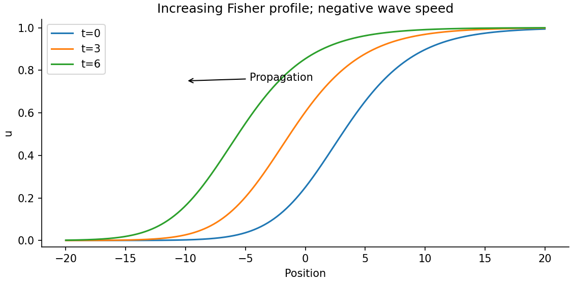
Let and with , . The profile equation is . Multiplication by and integration givesConsequently : the increasing front moves left, with the state invading . Linearization at its leading edge gives real monotone exponents only when , yielding the usual Fisher front speed range. A convenient exact example isSubstitution verifies it and the figure shows its leftward displacement. The source uses for the end limits after defining ; they denote the same spatial coordinate here.
Past exam of the topics in applied mathematics course of the University of Oxford 2010 A 1 b iii Solution by Codex 0 2026-10-31
Codex 0 2026-10-31Put . The harvested vector field is . Define the extinction threshold , and let be the positive local maximum of , with . Writing , givesPositive equilibria are intersections of with the horizontal line . A lower stable branch in exists exactly for . A pair in exists exactly for : its smaller member has and is unstable; its larger member has and is stable. At a positive root the linear eigenvalue is , which proves these claims. Extinction has eigenvalue , becoming stable for .
The harvested bistable population thresholds determine the behaviour. If , the upper stable population and its unstable separator first disappear in a saddle-node bifurcation. Populations then tend to the remaining lower stable state until that branch reaches extinction at ; beyond it extinction attracts every positive initial state. If , the lower stable branch reaches extinction first. For , extinction and the upper positive state are both stable, separated by the middle unstable root. Increasing effort through then destroys the remaining positive attractor, causing a sudden collapse to extinction. If , both events occur at the same effort at different populations.
At , near zero the leading term is , so extinction attracts from the physical right side algebraically, despite its zero linear eigenvalue. At , the double positive root is semistable: locally , attracting from above and repelling from below. These critical cases matter for exact initial data. The figure shows examples of both strict threshold orderings.
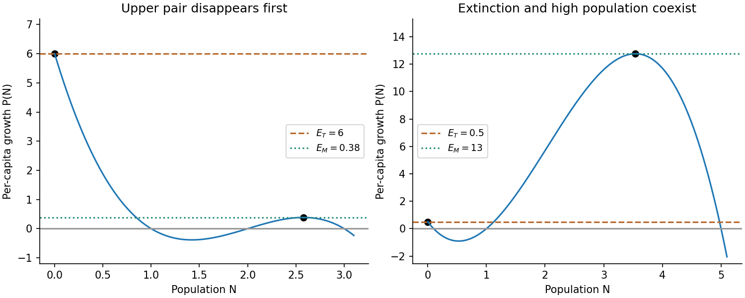
Two possible orderings of the extinction and saddle-node harvesting thresholds
. Details. Past exam of the topics in applied mathematics course of the University of Oxford 2010 A 1 b ii Solution by Codex 0 2026-10-31
Codex 0 2026-10-31The four nonnegative equilibria are . Since all factors are positive below , the sign of on consecutive intervals isThe phase line therefore points away from zero, towards , away from , and towards . Equivalently , and at each simple positive root , . Their signs alternate negative, positive, negative.
Hence extinction and are unstable, while and are asymptotically stable. Initial positive populations below tend to ; those above tend to ; an initial population exactly at remains there. This is bistability with a threshold separating the two basins.
Past exam of the topics in applied mathematics course of the University of Oxford 2010 A 1 b i Solution by Codex 0 2026-10-31
Codex 0 2026-10-31A steady population is a root . To linearize one needs differentiable near that root, an extra local regularity assumption beyond the source's continuity. Setting gives , hence at linear order.
Thus gives linear asymptotic stability and gives instability. If , linearization is inconclusive. In a one-dimensional phase line, the more general nonlinear test is whether the vector field points towards the root from both sides. At the physical boundary , only the right-hand side matters. Continuity alone does not guarantee uniqueness of trajectories, so a standard well-defined flow also presumes a local uniqueness condition, such as local Lipschitz continuity.
Past exam of the topics in applied mathematics course of the University of Oxford 2010 A 1 a iii Solution by Codex 0 2026-10-31
Codex 0 2026-10-31With constant-effort harvesting, the constant-effort model isThe extinction multiplier becomes , so extinction is linearly stable when . At its multiplier crosses . Values large enough to make the next population negative lie outside the physical validity of this untruncated harvest model.
Any positive fixed point solves . Since that ratio is strictly decreasing, there is at most one such point, and it decreases with effort. Differentiating the fixed-point equation yieldsIf the unharvested positive branch exists, it continues for and approaches zero as . This follows because its required ratio lies between and ; its intersection lies between zero and the unharvested fixed point. There is no positive fixed point for .
The positive-state multiplier is by concavity. It is stable precisely whenCrossing can change stability through a flip, but the direction of change is not fixed by the three assumptions: has no prescribed sign. In the illustrated saturating example, increasing effort eventually removes the positive branch at extinction. The finite upper stability bound for the algebraic extinction map should not be interpreted as a physically meaningful recovery of a population at unrealistically large harvest effort.
Past exam of the topics in applied mathematics course of the University of Oxford 2010 A 1 a ii Solution by Codex 0 2026-10-31
Codex 0 2026-10-31Let be a fixed point and put . Taylor expansion gives , so the linear perturbation is . Thereforeis the condition for linear asymptotic stability. A multiplier in gives monotone decay; one in gives alternating decay. If its magnitude exceeds one, perturbations grow. Magnitude one is nonhyperbolic and needs nonlinear analysis.
Strict concavity and already give . Thus the remaining stability requirement is . If is additionally nonnegative on the entire half-line, strict concavity prevents its derivative becoming negative there, since it would then force eventually negative. Under that stronger global population-map assumption the positive fixed point is automatically stable. The printed local slope and concavity information, without that global nonnegativity requirement, does not by itself rule out a flip instability.
Past exam of the topics in applied mathematics course of the University of Oxford 2010 A 1 a i Solution by Codex 0 2026-10-31
Codex 0 2026-10-31For this concave recruitment map, the extinction state is invariant because . Near extinction, with multiplier above one, so small positive populations initially grow. The strict concavity means marginal recruitment decreases as population increases. More precisely, for ,since . Thus per-capita recruitment decreases and the graph bends downwards from an initial slope greater than that of the identity line.
A positive fixed point, if present, is the unique positive intersection with : the strictly decreasing ratio can cross one at most once. The sketch shows the usual saturating example , which crosses at .
The three assumptions alone do not guarantee this crossing. For example satisfies all three and remains strictly above for every . An extra large-population restriction, such as somewhere, supplies existence. Keeping this distinction avoids inventing a carrying capacity that is not implied by the printed hypotheses.
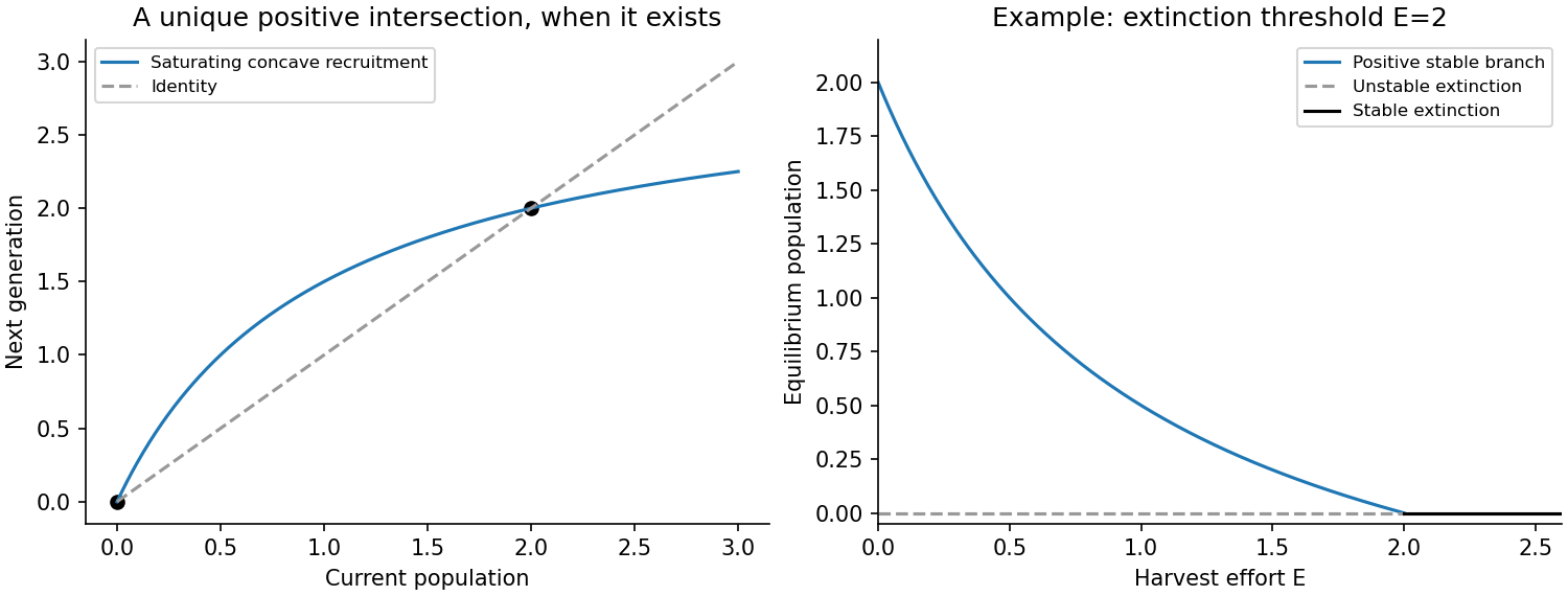
Concave recruitment and the identity line, with loss of the positive equilibrium under harvesting
. Details. Past exam of the topics in applied mathematics course of the University of Oxford 2009 B 4 b iii Solution by Codex 0 2026-10-31
Codex 0 2026-10-31The closed annulus is positively invariant by the radial signs, and excludes equilibria there. Poincaré-Bendixson therefore yields a periodic orbit. Its stability can be established explicitly rather than inferred merely from trapping.
For the exact anisotropic radial limit cycle, set . Then , or . Its unique periodic solution isIt is positive and stays within the trapping annulus. Any other solution at the same phase has , proving radial attraction and uniqueness of the positive periodic orbit. The full planar period is , since a full angular revolution takes that time; the half-turn symmetry of the radius does not halve the period of the position vector. The nontrivial return periodic-orbit multiplier is . Thus the periodic orbit is asymptotically stable, and all nonzero forward trajectories approach it up to phase.
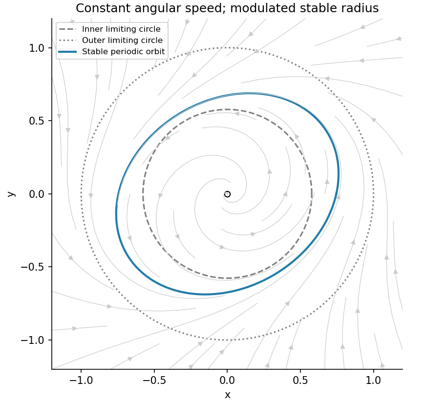
The trapping annulus and the explicitly attracting angularly modulated limit cycle
. Details. Past exam of the topics in applied mathematics course of the University of Oxford 2009 B 4 b ii Solution by Codex 0 2026-10-31
Codex 0 2026-10-31Use , with . Dotting the vector field with the radial direction and taking its angular cross-product givesThe angular factor ranges from one to three. Hence every radial component is outward for , and every radial component is inward for . The limiting radii areThere is a minor strictness point in the wording. At the outward inequality is non-strict, with tangencies where ; at the inward inequality is non-strict, with tangencies where . Thus these are the supremum and infimum for strict crossing at all angles. The weak inequalities at the endpoints are exactly what is needed for the closed trapping annulus in the next part.
Past exam of the topics in applied mathematics course of the University of Oxford 2009 B 4 b i Solution by Codex 0 2026-10-31
Codex 0 2026-10-31The cubic terms vanish in the linearization, leaving . Its eigenvalues are , so the origin is a repelling focus equilibrium. The nonzero imaginary part gives rotation, while the positive real part makes small amplitudes grow. In particular it cannot be the forward limit of nearby nonzero trajectories, which motivates looking for an attracting periodic orbit away from the origin.
Past exam of the topics in applied mathematics course of the University of Oxford 2009 B 4 a iii Solution by Codex 0 2026-10-31
Codex 0 2026-10-31For , the first integral isIts minimum occurs at the two centres. Levels between and give a periodic orbit around each centre equilibrium; positive levels give larger periodic orbits surrounding both wells. The zero level is the figure-eight separatrix through the saddle, with two homoclinic loops.
On , . The printed parametrization , , taking matching signs, satisfies this identity because . It also has and , so its parameter is physical reversed time, , rather than . It is nonetheless exactly a parametrization of the requested trajectory. In physical forward time one can use , on the right loop.
Approach to the origin requires , hence infinite physical time. Equivalently near the right-loop endpoint, so the elapsed time contains the divergent integral . The point at is reached in finite time from any interior point; it is the asymptotic saddle endpoints, not that turning point, that cause the infinite total traversal time.
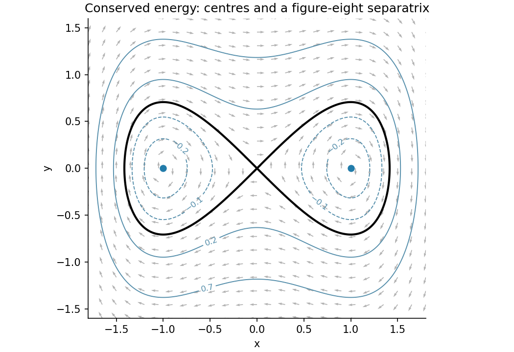
Double-well energy levels and the two homoclinic loops through the saddle
. Details. Past exam of the topics in applied mathematics course of the University of Oxford 2009 B 4 a ii Solution by Codex 0 2026-10-31
Codex 0 2026-10-31At either nonzero point the Jacobian matrix is , with eigenvaluesBoth points are attracting for and repelling for . For they are stable foci; for stable nodes. For they are unstable foci; for unstable nodes. At the two repeated-root boundaries they are degenerate nodes. At , linearization has purely imaginary eigenvalues; the conserved energy in the next part shows that they are actual nonlinear centres. Thus the zero-real-part case is resolved by an additional first integral, rather than by the linear test alone.
Pinned article: Introduction to the OurBigBook Project
Welcome to the OurBigBook Project! Our goal is to create the perfect publishing platform for STEM subjects, and get university-level students to write the best free STEM tutorials ever.
Everyone is welcome to create an account and play with the site: ourbigbook.com/go/register. We belive that students themselves can write amazing tutorials, but teachers are welcome too. You can write about anything you want, it doesn't have to be STEM or even educational. Silly test content is very welcome and you won't be penalized in any way. Just keep it legal!
Intro to OurBigBook
. Source. We have two killer features:
- topics: topics group articles by different users with the same title, e.g. here is the topic for the "Fundamental Theorem of Calculus" ourbigbook.com/go/topic/fundamental-theorem-of-calculusArticles of different users are sorted by upvote within each article page. This feature is a bit like:
- a Wikipedia where each user can have their own version of each article
- a Q&A website like Stack Overflow, where multiple people can give their views on a given topic, and the best ones are sorted by upvote. Except you don't need to wait for someone to ask first, and any topic goes, no matter how narrow or broad
This feature makes it possible for readers to find better explanations of any topic created by other writers. And it allows writers to create an explanation in a place that readers might actually find it.
Figure 1. Screenshot of the "Derivative" topic page. View it live at: ourbigbook.com/go/topic/derivativeVideo 2. OurBigBook Web topics demo. Source. - local editing: you can store all your personal knowledge base content locally in a plaintext markup format that can be edited locally and published either:This way you can be sure that even if OurBigBook.com were to go down one day (which we have no plans to do as it is quite cheap to host!), your content will still be perfectly readable as a static site.
- to OurBigBook.com to get awesome multi-user features like topics and likes
- as HTML files to a static website, which you can host yourself for free on many external providers like GitHub Pages, and remain in full control

Figure 2. You can publish local OurBigBook lightweight markup files to either OurBigBook.com or as a static website.
Figure 3. Visual Studio Code extension installation.
Figure 5. . You can also edit articles on the Web editor without installing anything locally. Video 3. Edit locally and publish demo. Source. This shows editing OurBigBook Markup and publishing it using the Visual Studio Code extension. 
- Infinitely deep tables of contents:




All our software is open source and hosted at: github.com/ourbigbook/ourbigbook
Further documentation can be found at: docs.ourbigbook.com
Feel free to reach our to us for any help or suggestions: docs.ourbigbook.com/#contact