The theorem givesIntegration by parts has zero boundary term: the sine vanishes at zero and the Gaussian tends to zero at infinity. Hence $F^{\prime }(t)=-2t{\int }_0^{\infty }{e}^{-x^2}\cos (2xt)dx=-2tF(t)$.

The same Gaussian majorant and dominated convergence give continuity at zero, where the allowed Gaussian integral gives $F(0)=\sqrt{\pi }/2$. The differential equation implies $(e^{t^2}F(t){)}^{\prime }=0$; continuity at zero fixes that constant. Thus

We first prove the differentiation theorem. Fix $t\in (0,b)$ and take nonzero $h\to 0$ with $t+h\in (0,b)$. The measurable difference quotientsconverge pointwise to $f_t(x,t)$. The mean value theorem and the assumed derivative bound give $|q_h(x)|\le g(x)$. In particular $f_t(\cdot ,t)$ is measurable as a limit of quotients along a sequence, and its bound by $g$ proves integrability. The dominated convergence theorem, in its parameter-limit form, says that pointwise convergence with a common integrable bound permits convergence of the integrals. Applying it yieldsThe parameter-limit statement follows from the ordinary sequential theorem by applying it to every sequence of nonzero $h$ tending to zero.

For the specific function, $|f(x,t)|\le e^{-x^2}$, which is integrable by the allowed fact. It is differentiable in $t$, withThe last majorant has integral one on $[0,\infty )$, using the substitution $u=x^2$. All three hypotheses therefore hold. The indicator of the parameter domain is one at every point under consideration and does not affect this derivative.

Take $a=[x]$. Every quotient class is a polynomial expression in $a$ with coefficients from $F$, so $K=F[a]$. Substitution gives $f(a)=[f(x)]=0$. ThusThis constructs a field containing a root even when no root existed in the original field.

Polynomial division gives a unique remainder of degree less than $n$ in every coset. Thus the classesspan the quotient as an $F$-vector space. A linear combination of them that vanishes would be a polynomial of degree less than $n$ divisible by $f$, so it is the zero polynomial. They are therefore linearly independent, proving

An irreducible polynomial has positive degree, so its ideal is proper: otherwise $1=fh$ would contradict degrees. Every nonzero class $[g]$ has a representative not divisible by $f$. Irreducibility gives $\gcd (g,f)=1$, and the Euclidean algorithm supplies polynomials $u,v$ with $ug+vf=1$. Passing to the quotient gives $[u][g]=1$. Thus the quotient is a nonzero commutative ring in which every nonzero element has an inverse, hence a field. Constants embed injectively because no nonzero constant lies in the positive-degree ideal $(f)$.

FactorThe roots are $\pm \sqrt{2},\pm i$, so the splitting field is $\mathbb{Q}(\sqrt{2},i)$. The real quadratic field $\mathbb{Q}(\sqrt{2})$ does not contain $i$, which adds a further degree two. Therefore

Let $\zeta =e^{\pi i/4}$. Its odd powers are exactly the four roots, so $\mathbb{Q}(\zeta )$ is the splitting field. The polynomial $x^4+1$ is irreducible: after the invertible substitution $x\mapsto x+1$, it becomes $x^4+4x^3+6x^2+4x+2$, which satisfies Eisenstein criterion at two. HenceEquivalently the field is $\mathbb{Q}(\sqrt{2},i)$, since $\zeta =(1+i)/\sqrt{2}$, ${\zeta }^2=i$ and $\zeta +{\zeta }^{-1}=\sqrt{2}$.

First address the general splitting-field request. A splitting field is an extension in which the polynomial factors into linear factors and which is generated over the base field by its roots. For a degree-$m$ polynomial, adjoin a root of an irreducible factor. The quotient construction in the preceding parts gives an extension of degree at most $m$. Remove the resulting linear factor and repeat, now with a polynomial of degree $m-1$ over that extension. Induction and the tower law giveThe resulting field is generated by the roots and is a splitting field. Repeated roots or inseparability can only reduce the required degrees; separability was not used.

For the specified cubic, put $a=\sqrt[3]{2}$ and $\omega =e^{2\pi i/3}$. Its splitting field is $\mathbb{Q}(a,\omega )$. Eisenstein criterion at two gives $[\mathbb{Q}(a):\mathbb{Q}]=3$. This cubic field is real and therefore does not contain the nonreal $\omega$, whose quadratic polynomial is $x^2+x+1$. Consequently

For the positive-direction alternative, use the same paired statistic $t_{\mathrm{obs}}=2.607/(4.713/\sqrt{15})$, but reject at level $\delta$ only when $t_{\mathrm{obs}}>t_{14,1-\delta }$. Its one-sided $p$-value isBecause the observed mean difference is positive and the null Student probability distribution is symmetric, the two-sided $p$-value is twice this upper-tail probability, consistent with the supplied $0.05$ and $0.025$.

The two-sided value is the null-model probability of a test statistic at least as far from zero in either direction as the observation. The one-sided value uses only the direction of larger cross-fertilized heights. They are probabilities under the assumed null sampling distribution, not posterior probabilities that the null hypothesis is true.

At the reported precision, the two-sided result is on the conventional 5 percent boundary; rounding can matter for a strict numerical threshold. The one-sided result is significant at5 percent and supports a positive mean difference if that directional alternative was chosen in advance. Choosing the direction after observing the sign would not justify using the smaller one-sided probability as a prespecified test. The paired design controls shared pot conditions, while the inference still relies on the independence and probability distribution assumptions for the differences.

For a sample of size $n\ge 2$, defineFor the zero-mean Gaussian sample, the standardized vector $(X_1/\sigma ,\dots ,X_n/\sigma )$ has independent standard normal coordinates. Apply an orthogonal transformation whose first row is $(1,\dots ,1)/\sqrt{n}$. The resulting coordinates $Z_1,\dots ,Z_n$ remain independent standard normals: their joint density depends only on squared Euclidean length and the transformation has unit absolute Jacobian. Its first coordinate is $Z_1=\sqrt{n}\overline{X}/\sigma$, while orthogonal decomposition givesThusThe ratio of the first independent standard normal and the square root of the normalized chi-square variable has a Student probability distribution, giving

For the paired height observations, form one cross-minus-self difference per pot. The sampling units for this test are the fifteen differences, not thirty separate plant heights. Under the usual independent normal model for differences, a null mean of zero gives a $t_{14}$ statistic. The observed statistic isFor the two-sided alternative, reject at significance level $\delta$ if $|t_{\mathrm{obs}}|>t_{14,1-\delta /2}$. Its two-sided $p$-value is $2[1-F_{t_{14}}(|t_{\mathrm{obs}}|)]$. This uses the recorded values without performing the numerical calculation forbidden by the question. The normal difference model is what makes the small-sample Student calibration exact.

Assume $N\ge 2$, as required by the source's selection probabilities, and put $q=(1-p)/(N-1)$. Conditional on the red book's current position, the next independent selection determines its move without needing its earlier history. Selecting the red book moves it left, unless already leftmost. Selecting the plain book immediately to its right moves it right. Every other selection leaves its position unchanged. Thus this position process is a Markov chain on $\{1,\dots ,N\}$, withand boundary self-loop probabilities $P_{11}=1-q$, $P_{NN}=1-p$. These account for every selection and each row sums to one.

Stationarity at the first state gives ${\pi }_1=(1-q){\pi }_1+p{\pi }_2$, hence $p{\pi }_2=q{\pi }_1$. When $N\ge 3$, for the second state substitution of this identity into its stationarity equation gives $p{\pi }_3=q{\pi }_2$. More generally, summing stationarity over the initial segment $\{1,\dots ,i\}$ equates its sole outward and inward probability flows:Write $r=q/p$. Then ${\pi }_i={\pi }_1{r}^{i-1}$. Normalization givesThe expression is positive also for $r>1$, since both numerator prefactor and denominator are negative. The uniform case is exactly $p=1/N$, when all books are equally likely to be selected. Since both neighboring transition probabilities are positive, the finite chain is irreducible; the displayed stationary distribution is therefore unique.

Starting from a state $i$, let ${\tau }_i=\inf \{n\ge 1:X_n=i\}$ be the first return time, with value infinity if no return occurs. The state is recurrent if ${\mathrm{Pr}}_i({\tau }_i<\infty )=1$ and transient if this probability is less than 1. A recurrent state is positive recurrent if ${\mathbb{E}}_i{\tau }_i<\infty$, and null recurrent if that expectation is infinite.

If $i$ and $j$ communicate, choose $r,s$ with $p_{ij}^{(r)}>0$ and $p_{ji}^{(s)}>0$. The Chapman-Kolmogorov equations give, for every $n$,If $j$ is recurrent, the supplied criterion makes ${\sum }_n{p}_{jj}^{(n)}$ infinite. Summing this inequality shows that ${\sum }_n{p}_{ii}^{(n)}$ is also infinite, so $i$ is recurrent. The same argument with the states exchanged gives the converse. Hence recurrence and transience are class properties: states in one communicating class cannot have different answers to that dichotomy.

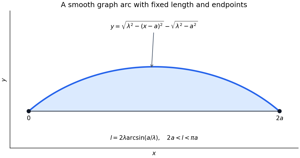
For the upper function graph, the vertical cross-section of the enclosed region has length $y(x)$, so its area is $J[y]={\int }_0^{2a}y(x)dx$. A maximizing nonnegative arch therefore uses $F=y$ and $G=\sqrt{1+y^{\prime 2}}$ in the normal Euler-Lagrange equation. It becomesIntegrating once gives $y^{\prime }/\sqrt{1+y^{\prime 2}}=(c-x)/\lambda$. The concave upper branch has $\lambda >0$ and integrates to $y=\sqrt{{\lambda }^2-(x-c{)}^2}+d$. The equal zero endpoint heights force $c=a$ and $d=-\sqrt{{\lambda }^2-a^2}$. HenceIt is a circular arc. To find its parameter, substitute into the length integral: $\sqrt{1+y^{\prime 2}}=\lambda /\sqrt{{\lambda }^2-(x-a{)}^2}$, givingThis scalar equation determines $\lambda$ numerically when needed; no explicit solution is required.

The arch is a global maximum in its smooth function graph regime. For $\lambda >0$, the integrand $y-\lambda \sqrt{1+y^{\prime 2}}$ is concave and strictly concave in its slope. Its supporting-tangent inequality, integrated against any competing function graph with the same endpoint values, has first-order term zero by the Euler-Lagrange equation. Thus $J[y]-\lambda I[y]\le J[y_{\ast }]-\lambda I[y_{\ast }]$. On the fixed-length class this is $J[y]\le J[y_{\ast }]$; strict slope concavity also gives uniqueness.

The source leaves the length range implicit. A twice continuously differentiable function graph of this form needs $\lambda >a$, giving $2a<l<\pi a$. At $l=2a$ the straight function graph is the degenerate solution. The semicircle limit $l=\pi a$ has vertical endpoint tangents and is outside that smooth function graph class. For $l>\pi a$, no arc in the claimed smooth function graph family exists, so the stated formula cannot describe a twice continuously differentiable maximizing function graph under those unrestricted data. Allowing overhanging curves changes the admissible class.

Write $I[y]={\int }_a^{b}G(x,y,y^{\prime })dx$. For endpoint-zero variations $\eta$, the first variations areFor a normal constrained extremal, choose a variation ${\eta }_0$ with $\delta I({\eta }_0)\ne 0$. Given any $\eta$, use the implicit function theorem to choose a small correction in the ${\eta }_0$ direction so that $y+t\eta +s(t){\eta }_0$ preserves the constraint. Differentiating it and the stationarity condition at zero givesIntegrate the derivative-of-variation term by parts. Since the variations vanish at both endpoints, the boundary term is zero. The fundamental lemma of the calculus of variations then givesThe regularity condition on the constraint is what permits the coefficient of $F$ to be normalized to 1. In a degenerate case, the general multiplier statement uses ${\lambda }_{0}F-{\lambda }_{1}G$ with the two coefficients not both zero; the source's displayed form is the normal case.

For a string described as a function graph $r(x)=(x,y(x))$, its arc-length element is $|r^{\prime }(x)|dx=\sqrt{1+y^{\prime }(x{)}^2}dx$. Inextensibility therefore givesThis also forces $l\ge 2a$, with equality only for the straight function graph.

For fixed real $t$, multiplication by $e^{itx}$ does not change the absolute value. The product integrability proved in (ii) therefore justifies Fubini theorem in the following calculation. Set $u=x-y$ in the inner integral:ThusThe positive exponential convention in the source is used throughout; no normalization factor is introduced under that convention.

Choose measurable versions of the two Lebesgue integrable functions and consider $F(x,y)=g(x-y)h(y)$. Translation and the corresponding linear change of variables preserve Lebesgue measurability; one can first use Borel versions and then disregard the resulting null-set changes. Tonelli's theorem and translation invariance giveFubini theorem therefore shows that the section in $y$ is integrable for almost every $x$. Define $(g\ast h)(x)$ by that section integral where it exists and by zero on the exceptional null set. Fubini theorem also makes this a measurable Lebesgue integrable function, withIts almost-everywhere defining formula is precisely the desired convolution. This construction explains why an everywhere-existing pointwise integral is not required.

Fubini's theorem for the product of two sigma-finite measure spaces states that an integrable measurable function on the product has integrable sections almost everywhere, the section integrals define Lebesgue integrable functions, and both iterated integrals equal the product integral. The integrability hypothesis is absolute integrability. For nonnegative measurable functions, Tonelli's theorem gives equality of the possibly infinite product and iterated integrals without first assuming finiteness.

The displayed function is not Lebesgue integrable. Its value at the origin can be assigned arbitrarily, since a point is a null set. On $0<x<1$ and $0<y<x/2$,Consequently Tonelli's theorem gives the divergent lower boundThe signed iterated integrals illustrate why the hypothesis matters. For $x>0$, $f(x,y)={\partial }_y[y/(x+y{)}^2]$, so integration first in $y$ and then in $x$ gives $1/2$. Integrating first in $x$ gives $-1/2$, using $f(x,y)=-{\partial }_x[x/(x+y{)}^2]$. Exceptional boundary sections have measure zero. Thus finite iterated values do not establish product integrability.

Use $|\sin (\alpha x)|\le |\alpha |x$ for $x\ge 0$. For the source's functions,The last integral follows by the substitution $u=nx$ and integration by parts. Since ${\sum }_n{n}^{-2}$ converges, (ii) permits summing the integrals and identifies an integrable almost-everywhere sum.

For every $x>0$, the geometric series givesThe functions vanish on $x\le 0$, and the single endpoint does not change the integral. Use the supplied integral of $f_n$ to obtainThe estimates include negative $\alpha$ through its absolute value, and the case $\alpha =0$ gives zero on both sides.

Put $G_N={\sum }_{n=1}^N|f_n|$. These are nonnegative measurable functions increasing to $G={\sum }_{n=1}^{\infty }|f_n|$, possibly initially with value infinity. Monotone convergence theorem givesAn infinite value on a set of positive measure would force an infinite integral. Thus $G$ is finite almost everywhere and, after setting it to zero on its null exceptional set if desired, is integrable.

Where $G$ is finite, the real series ${\sum }_n{f}_n$ is absolutely convergent. Define its sum to be $h$ there and zero on the exceptional null set. Measurability follows as an almost-everywhere limit of partial sums, and $|h|\le G$ almost everywhere gives integrability. Every partial sum is dominated by $G$, so dominated convergence theorem yieldsIn fact the convergence is also in the integrable-function norm:

The monotone convergence theorem says that if $0\le f_n\uparrow f$ almost everywhere and the functions are measurable on a measure space, thenwith infinite integrals permitted. The limit is measurable after the usual modification on any exceptional null set.

The dominated convergence theorem says that if measurable functions $f_n$ converge almost everywhere to $f$ and satisfy $|f_n|\le g$ almost everywhere for an integrable nonnegative function $g$, then $f$ is integrable andThe theorem applies equally to real or complex functions. In particular domination must be by one fixed Lebesgue integrable function, rather than by a different bound for each $n$.