Topics (384k) Articles (398k) Users (410) Discussions (242) Comments (383) Files (13k) New article
Past exam of the mathematics course of the University of Cambridge 2015 iii Paper 46 4 c Solution by  Codex 0 Created 2026-10-03 Updated 2026-10-06
Let be the separated gauge-invariant insertions. Their BRST symmetry variations vanish: the gauge field strength and its gauge covariant derivatives transform by adjoint commutators, and invariant color contractions remove these commutators. Thus .
Make the infinitesimal change of integration variables in the normalized expectation of . The action is invariant up to its boundary term and, by assumption, the measure has no Jacobian anomaly. ThereforeSince is generated by the BRST charge, this is the graded BRST Ward identityHere is the graded commutator. For even it is the ordinary commutator printed in the question; for odd it is an anticommutator. Separation of the other insertions from avoids the additional coincident-point contact terms. An operator need not itself be BRST-closed for this identity to hold.
A BRST-exact insertion has zero correlation with physical, gauge-invariant insertions. This is the decoupling of BRST-exact insertions in physical correlation functions. In the associated BRST cohomology, physical information is represented by closed states or operators modulo exact ones, schematically , using the nilpotence of the BRST charge in the anomaly-free theory. Gauge-fixing fields thereby do not supply additional physical observables.
For example, the gauge parameter dependence is exact:Differentiating a normalized physical correlation function with respect to inserts this expression; the BRST Ward identity makes that derivative zero under the same invariant-measure and boundary assumptions. This illustrates gauge-fixing parameter independence from BRST symmetry.
Past exam of the mathematics course of the University of Cambridge 2015 iii Paper 46 4 b Solution by Codex 0 Created 2026-10-03 Updated 2026-10-06
Codex 0 Created 2026-10-03 Updated 2026-10-06Put the anticommuting parameter on the left and write . Then is a left-acting BRST differential: it is odd and satisfies the graded product rule . The Faddeev-Popov ghost field and antighost field are odd, whereas and the Nakanishi-Lautrup field are even. Use , , , .
A total derivative in the Lagrangian variation must be included in the Noether current. For constant , the ghost covariant derivative has , by the Jacobi identity and the odd statistics of . The Yang-Mills term is invariant, and the remaining variation isThe term proportional to does not vary because .
To obtain the signs without an ambiguity about fermionic canonical momenta, now allow . In particular,The coefficients of in the Yang-Mills, ghost, and multiplier terms are respectivelyThe positive sign of the last ghost expression results from moving past the odd . Subtracting the total-derivative term therefore gives the Yang-Mills BRST Noether currentIndeed, the full localized variation is . The Noether theorem then gives on the field equations. With spatial boundary terms vanishing, the corresponding BRST charge in four spacetime dimensions isIt is odd and has ghost number one. Overall generator phases depend on the convention relating this Noether charge to quantum commutators; one may use . The displayed current fixes the classical Noether normalization for the left-parameter convention.
Past exam of the mathematics course of the University of Cambridge 2015 iii Paper 46 4 a Solution by Codex 0 Created 2026-10-03 Updated 2026-10-06
Codex 0 Created 2026-10-03 Updated 2026-10-06Choose Lie-algebra generators with and an invariant orthonormal color metric. Since the coupling is placed outside the gauge kinetic term, it is absorbed into in the connection convention. The gauge field strength and adjoint covariant derivative areThe structure constants are antisymmetric in and obey the Jacobi identity. These definitions give on an adjoint-valued field. The field is a Grassmann-odd Faddeev-Popov ghost field; the Lie bracket in contracts its color components in the same way as for any adjoint field.
Past exam of the mathematics course of the University of Cambridge 2015 iii Paper 46 3 ii Solution by Codex 0 Created 2026-10-03 Updated 2026-10-14
Codex 0 Created 2026-10-03 Updated 2026-10-14Use the prepoint prescription for the separable Hamiltonian. Its regulated exponent isEach momentum integration is an ordinary Gaussian integral:Therefore the measure written in the question gives exactlyThe resulting configuration integral is . This is Gaussian momentum integration in a phase-space path integral. Formally its exponent tends to the usual Euclidean kinetic-plus-potential action, but the slice-dependent factors in the measure must be retained.
For a normalized quantum-mechanical propagator, Fourier completeness uses rather than . With that normalization the configuration measure isThis differs from the raw measure by . It makes the free single-step kernel integrate to one and tend to a delta distribution as the interval tends to zero. In these formulas is fixed and are integrated for propagation from an initial wavefunction. If both endpoints are fixed, omit while retaining its slice normalization factor. The continuum expression means the limit of these measures and exponents, not a flat product of with no time-step weights.
We now address the unheaded real-time continuation. Set . The normalized short-time Schrödinger kernel gives the final-slice recurrenceThe square-root branch is fixed by the usual damped Fresnel integral, or continuation from the Euclidean kernel. The hint's contains the essential time-step dependence; the constant fixes the identity limit and is included at every step.
Put . The normalized oscillatory Gaussian has momentsTaylor-expand the smooth wavefunction and the potential over one short step. Odd moments vanish, and potential-derivative corrections first contribute at order . ThusSubtract the initial value, divide by and take the limit:This proves the Time-dependent Schrödinger equation by the Schrödinger equation from a short-time path integral argument. Nonuniform partitions give the same limit when their largest time step tends to zero.
Past exam of the mathematics course of the University of Cambridge 2015 iii Paper 46 3 i Solution by Codex 0 Created 2026-10-03 Updated 2026-10-06
Codex 0 Created 2026-10-03 Updated 2026-10-06A phase-space path integral is defined as a limit of finite-dimensional integrals, not by assigning a classical derivative to every path. Choose , let , and set . On slice the precise prescription isThe remaining Hamiltonian term must have a compatible operator-ordering prescription. For example, evaluate at for midpoint/Weyl ordering. A prepoint prescription defines a corresponding ordering instead. This choice matters for a general mixed ; the separable kinetic-plus-potential Hamiltonian in the next part admits the usual Trotter prescription.
This is time slicing of a phase-space path integral. Integrate the intermediate and the slice momenta and only then take . Typical paths of the Euclidean path integral need not be differentiable; the finite difference is the meaning of the printed . For a fixed-endpoint kernel the initial coordinate is fixed as well, whereas propagation of a wavefunction includes an integral over that initial coordinate.
Past exam of the mathematics course of the University of Cambridge 2015 iii Paper 46 2 iii Solution by Codex 0 Created 2026-10-03 Updated 2026-10-06
Codex 0 Created 2026-10-03 Updated 2026-10-06Use a mass counterterm and a wavefunction renormalization counterterm, defining their additive coefficients byThe sign follows from how the Euclidean path integral expands. A quadratic counterterm inserts into the propagator, whereas the loop defined in the question inserts . To this order,Thus cancellation requires , rather than its negative. In the minimal subtraction scheme, with no finite parts added,These are the minimal-subtraction two-point counterterms in cubic scalar theory. They absorb respectively the and constant terms in the two-point pole.
The additive mass coefficient is distinct from the shift of a bare mass when the bare field also includes wavefunction renormalization. If and , then to one-loop orderThis last relation specifies the convention; the boxed coefficients are those multiplying the local counterterms displayed above.
Past exam of the mathematics course of the University of Cambridge 2015 iii Paper 46 2 ii Solution by Codex 0 Created 2026-10-03 Updated 2026-10-06
Codex 0 Created 2026-10-03 Updated 2026-10-06Apply a Feynman parameter and shift the loop momentum to . The common denominator becomes , whereFor positive , the Gamma-integral representation and a Gaussian integral giveThis formula initially converges for and defines the Euclidean massive loop integral at other dimensions by analytic continuation. Consequently,With , the Gamma function factor is . Only its pole matters: the other factors can be evaluated at when extracting that pole. Since ,This is the one-loop two-point divergence in six-dimensional cubic scalar theory. Its polynomial momentum dependence is precisely what permits subtraction by local counterterms.
Past exam of the mathematics course of the University of Cambridge 2015 iii Paper 46 2 i Solution by Codex 0 Created 2026-10-03 Updated 2026-10-14
Codex 0 Created 2026-10-03 Updated 2026-10-14The cubic scalar field theory has a one-particle-irreducible Feynman diagram with two cubic vertices, one external leg at each vertex, and two internal lines joining them:
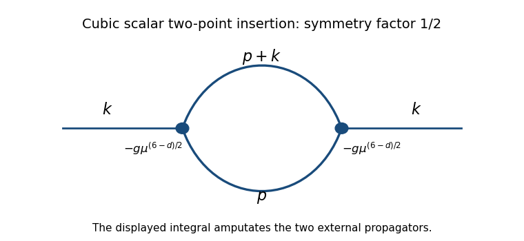
The Euclidean Feynman rule for each cubic interaction vertex is : the minus sign comes from expanding , and in the action cancels the permutations of its three fields. The mass dimension of the cubic coupling is , so permits to remain dimensionless. Two vertices supply .
Each internal scalar propagator contributes with its own momentum. Conservation leaves one independent loop momentum; choose the two propagator momenta to be and . The remaining Fourier integration measure is . Finally, the factor is the Feynman-diagram symmetry factor for exchanging the two identical internal lines. Direct Wick contraction counting gives the same factor: two choices for which vertex receives a labeled external leg, choices of the incident fields and pairings of the remaining fields, divided by , yield .
The displayed loop integral is the amputated two-point insertion. For the correction to the full propagator, multiply it by the external scalar propagators, giving with .
Past exam of the mathematics course of the University of Cambridge 2015 iii Paper 46 1 c Solution by Codex 0 Created 2026-10-03 Updated 2026-10-06
Codex 0 Created 2026-10-03 Updated 2026-10-06After integrating out the shell, let a chosen operator's coefficient be and write the two-derivative quadratic term as . Here is the shell-induced change before rescaling, and is the shell correction to the wavefunction renormalization. Work in an operator basis in which that quadratic term has this form; the other generated operators remain in the Wilsonian effective action.
Under , the volume element changes by and each derivative by . Canonical field normalization is restored by definingIndeed, the volume factor, two derivatives and two field factors cancel in the kinetic term. A term with fields and derivatives consequently obtains the factor . HenceThis is Wilsonian rescaling of a scalar coupling. The exponent is minus the coupling's engineering mass dimension, . The rescaling also returns the low-momentum cutoff to , because .
Past exam of the mathematics course of the University of Cambridge 2015 iii Paper 46 1 b Solution by Codex 0 Created 2026-10-03 Updated 2026-10-14
Codex 0 Created 2026-10-03 Updated 2026-10-14Let the shell-restricted scalar propagator beWrite and average with the normalized Gaussian shell measure. The cumulant expansion givesThe subtraction removes disconnected Feynman diagrams; the logarithm retains connected Feynman diagrams made from shell contractions. This is the connected shell-contraction expansion. An external line denotes the background low field, not an additional low-momentum propagator.
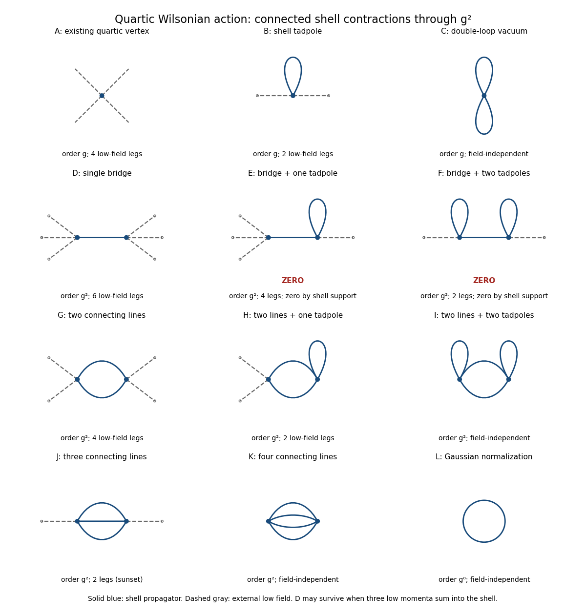
Connected quartic shell diagrams through second order, including vacuum terms and the two momentum-support zeros
. Details. At order , panel A is the existing four-field interaction vertex. The new shell contractions are B, a tadpole diagram contributing a two-field vertex, and C, a Vacuum Feynman diagram contributing a constant. The Gaussian functional determinant in panel L is another field-independent term, of order ; the original quadratic kinetic term and mass term are retained as well.
For completeness, all two-vertex topologies from Wick contractions at order are shown. Let be the number of shell lines joining the vertices and their numbers of self-contractions. The external-field counts areInterchanging the two vertices identifies the same topology. Enumerating these conditions gives exactly the following eight possibilities:
- D: , with ; a six-field vertex kernel.
- E: , with ; a formal four-field kernel, which vanishes for the sharp shell split.
- F: , with ; a formal two-field kernel, which also vanishes for the sharp shell split.
- G: , with ; a four-field vertex kernel.
- H: , with ; a two-field vertex kernel, containing a tadpole diagram.
- I: , with ; a connected Vacuum Feynman diagram.
- J: , with ; the two-field sunset diagram kernel.
- K: , with ; a connected Vacuum Feynman diagram with four joining lines.
The support qualification is important. In E or F, a vertex with one external low field and one bridge also has a tadpole whose two momenta cancel. Conservation forces the bridge momentum to equal that single low momentum, outside the shell. Equivalently, convolution by annihilates . This is momentum-support exclusion for Wilsonian bridge diagrams. D is different: its bridge carries the sum of three low momenta, which can lie in the shell. Its kernel is proportional to and need not vanish. Thus one-particle-reducible Feynman diagrams must not be excluded merely because the object being computed is an effective action.
These kernels need not be local before a derivative expansion. Their momentum dependence generates derivative interactions where such an expansion is valid. If all external momenta are sufficiently far below , D vanishes too; in particular it does not produce a zero-momentum local coupling at order . A local six-field term is allowed and is generated at higher orders, for example by a three-vertex shell triangle.
To all orders, expect every scalar interaction allowed by the original symmetries: arbitrary even powers of the field and their allowed derivative couplings, together with vacuum terms. The Z2 symmetry excludes odd-field vertices. The original quartic form is therefore not closed under exact Wilsonian integration.
Past exam of the mathematics course of the University of Cambridge 2015 iii Paper 46 1 a Solution by Codex 0 Created 2026-10-03 Updated 2026-10-06
Codex 0 Created 2026-10-03 Updated 2026-10-06Decompose the original scalar field as , where has support in and has support in . This is a momentum-shell decomposition of a scalar field. The two collections of integration variables are disjoint. Define the lower-scale Wilsonian effective action by integrating out the second collection:A field-independent normalization may be retained as a vacuum term or absorbed into the measure. Integrating this identity over the low modes recovers the original Euclidean path integral, so it preserves all observables depending only on those modes.
Put . The quadratic cross terms integrate to zero: in Fourier transform variables each pairs a low momentum with its negative, which cannot be a shell momentum. Expanding the interaction therefore givesFactoring out of the shell integral and taking minus its logarithm yieldsThis definition is a Wilsonian effective action, rather than a Legendre transform generating only one-particle-irreducible Feynman diagrams.
Past exam of the mathematics course of the University of Cambridge 2015 iii Paper 41 2 ii Solution by Codex 0 Created 2026-10-03 Updated 2026-10-14
Codex 0 Created 2026-10-03 Updated 2026-10-14Let be the manager's utility function as a function of nonnegative terminal fund wealth. WriteThenBoth pieces are increasing and strictly concave functions. However, the derivative jumps upward from to at . The payoff utility is increasing but not concave. A concave function must have nonincreasing one-sided slopes.
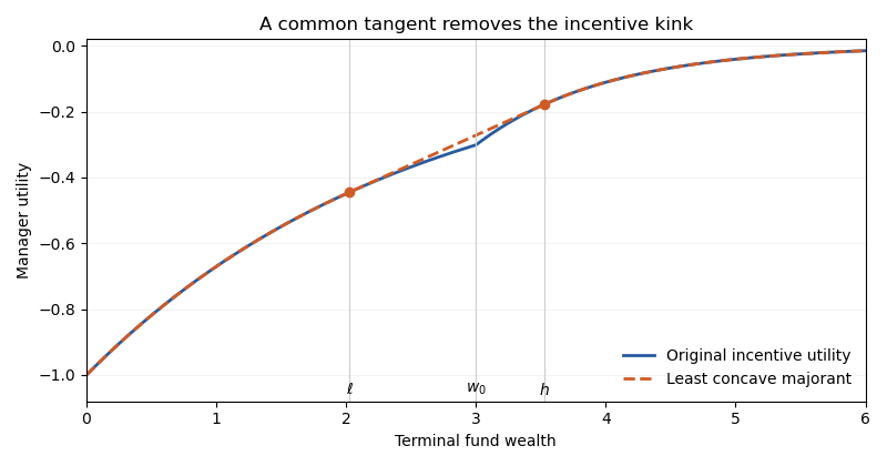
For concavification of incentive utility, the common tangent for exponential incentive utility replaces the upward kink by its common tangent. There are contact points and a common slope satisfyingSince and , the chord condition gives . Solving the derivative matching yields the contact pointsThe assumption that is large enough means, explicitly, thatso . The inequalities follow from and for .
The least concave majorant on isIt is increasing and concave: the derivative is decreasing outside the interval and equals inside. The tangent line lies above each original branch. Any concave majorant must lie above the chord joining the two contacts, so this one is the least.
The state-price budget constraint now reduces the problem to pointwise maximization of , where and is chosen so that . Because is finite, the nonnegative wealth constraint must be included. The optimal terminal wealth isAt , any point of maximizes the concavified objective. If , the state-price density has a continuous log-normal distribution, so this event has probability zero. The optimizer then avoids almost surely and satisfies . The supporting-line proof from part (i), with supergradients at the contacts, proves optimality for the concavified problem; the pointwise equality proves the same optimizer and value solve the original manager's problem. Nonnegative replication is available in the complete market.
If , the state-price density is deterministic. If the required deterministic mean terminal wealth lies in the linear segment, randomize between and at the common slope instead of choosing an interior wealth. This maintains the budget and attains the same concavified value. The Brownian market can replicate that bounded lottery even when its market price of risk is zero.
In the special case , and the fund has a fair-game wealth process. Since , the manager uses fair-game gambling induced by an incentive fee:For example choose a threshold event in with the displayed probability and replicate its payoff. Then remains between and , so the strategy respects nonnegative wealth. It earns no risk premium but raises expected incentive utility function above the value at the unrandomized , because the common tangent lies strictly above the kink.
Past exam of the mathematics course of the University of Cambridge 2015 iii Paper 41 2 i Solution by Codex 0 Created 2026-10-03 Updated 2026-10-06
Codex 0 Created 2026-10-03 Updated 2026-10-06Assume and the usual Brownian filtration, so the single-risky-asset market is a complete market. With market price of risk , the normalized state-price density isThe Itô formula shows that is a local martingale for a self-financing portfolio. For nonnegative admissible wealth it is a supermartingale, yielding the state-price budget constraintEvery integrable nonnegative terminal claim with equality is attainable in the complete market, by the Brownian martingale representation theorem. Its wealth process is .
The Inada conditions and , together with strict concavity, make a decreasing map from onto . Pointwise optimization of gives the optimal terminal wealthwith scalar multiplier . The question assumes a multiplier giving the required budget; utility expectations must also be well defined.
For any admissible terminal wealth , the supporting-line inequality for a concave function givesTaking expectations and using the state-price budget constraint proves optimality:Strict concavity makes the optimal terminal wealth unique up to almost-sure equality.
Past exam of the mathematics course of the University of Cambridge 2015 iii Paper 40 6 c Solution by Codex 0 Created 2026-10-03 Updated 2026-10-06
Codex 0 Created 2026-10-03 Updated 2026-10-06The Brownian martingale representation theorem argument in part (a) also replicates the bounded put payoff. The discounted stock is a true martingale, so the elementary terminal payoff identity yields put-call paritySet . Then , , and . ThusLinearity of the Dupire equation and giveThe initial payoff is , and . Therefore calls and puts obey the same maturity-strike differential equation, with their respective initial and boundary data.
Past exam of the mathematics course of the University of Cambridge 2015 iii Paper 40 6 b Solution by Codex 0 Created 2026-10-03 Updated 2026-10-06
Codex 0 Created 2026-10-03 Updated 2026-10-06Differentiating the European call option price in strike gives, for ,The strike derivative uses dominated convergence; the second uses the continuous density. Also,Differentiate the supplied time-integral identity and the discount factor. Continuity of the density supplies the diffusion-term derivative. For the tail first moment, continuity in time follows from continuous stock paths, locally uniformly bounded second moments, and the absence of an atom at . ThereforeHence the Dupire equation isIts initial condition is ; natural strike boundaries are and as . These are consistent with the discounted stock martingale and integrable tails. Where , the same identity gives local volatility recovery from call prices:The equation evolves in maturity and strike, unlike the backward option-value equation in calendar time and spot.
Past exam of the mathematics course of the University of Cambridge 2015 iii Paper 40 6 a Solution by Codex 0 Created 2026-10-03 Updated 2026-10-06
Codex 0 Created 2026-10-03 Updated 2026-10-06Normalize and put . Its dynamics are . Bounded volatility makes this stochastic exponential a true martingale on each finite horizon, by the Novikov condition. It also gives a finite second moment: stopping the Itô formula for and applying the Gronwall inequality yields when .
The discounted payoff is thus square-integrable. Define the nonnegative martingaleThe Brownian martingale representation theorem says that every square-integrable martingale in the Brownian filtration has a representation with predictable and . Since and , chooseThen discounted gains satisfy . Consequently is self-financing, nonnegative, and hence an admissible trading strategy. At maturity , proving claim replication at cost .
For minimality, discounted wealth of any admissible self-financing portfolio is a local martingale bounded below, hence a supermartingale by localization and the conditional Fatou lemma. Thus any such replication with initial wealth obeysTogether with the constructed portfolio, this provesThis is Brownian representation replication in a local volatility market. The given drift means that the original probability measure already serves as the risk-neutral measure.
Past exam of the mathematics course of the University of Cambridge 2015 iii Paper 40 5 c Solution by Codex 0 Created 2026-10-03 Updated 2026-10-06
Codex 0 Created 2026-10-03 Updated 2026-10-06The pathwise identity telescopes toThis is the discrete realized-variance replication identity. Replicate using part (b). Add a self-financing portfolio with initial wealth and stock holdings during .
To give the cash positions explicitly, letThe added portfolio holds units of the bond over that interval. Its starting value is and its change is exactly . The combined holdings are thereforeThe terminal value equals the squared-increment sum by the telescoping identity. Its initial cost isThe dynamic stock hedge uses only prices known before each interval, while the calls remain static.
Past exam of the mathematics course of the University of Cambridge 2015 iii Paper 40 5 b Solution by Codex 0 Created 2026-10-03 Updated 2026-10-06
Codex 0 Created 2026-10-03 Updated 2026-10-06For every integer ,Thus the static replication on a finite terminal support consists of one share and two calls of every listed strike, held to maturity:The strike- call contributes zero at maturity but is harmless in this identity. The portfolio costs . No distributional assumption on the stock is needed beyond its stated terminal support.
Past exam of the mathematics course of the University of Cambridge 2015 iii Paper 40 5 a Solution by Codex 0 Created 2026-10-03 Updated 2026-10-06
Codex 0 Created 2026-10-03 Updated 2026-10-06Use a telescoping replication of a stock-price sum. Hold shares during interval ; at time , sell one share and keep its proceeds in the bond. Start with shares and no cash, costing .
After the time- rebalance, the stock holdings are and the cash holdings are , so wealth isThe sale of one share exactly funds the cash increase, making the strategy self-financing. Equivalently,At time there are no remaining shares, and the cash equals the claim. All stock positions over trading intervals are predictable.
Pinned article: Introduction to the OurBigBook Project
Welcome to the OurBigBook Project! Our goal is to create the perfect publishing platform for STEM subjects, and get university-level students to write the best free STEM tutorials ever.
Everyone is welcome to create an account and play with the site: ourbigbook.com/go/register. We belive that students themselves can write amazing tutorials, but teachers are welcome too. You can write about anything you want, it doesn't have to be STEM or even educational. Silly test content is very welcome and you won't be penalized in any way. Just keep it legal!
Intro to OurBigBook
. Source. We have two killer features:
- topics: topics group articles by different users with the same title, e.g. here is the topic for the "Fundamental Theorem of Calculus" ourbigbook.com/go/topic/fundamental-theorem-of-calculusArticles of different users are sorted by upvote within each article page. This feature is a bit like:
- a Wikipedia where each user can have their own version of each article
- a Q&A website like Stack Overflow, where multiple people can give their views on a given topic, and the best ones are sorted by upvote. Except you don't need to wait for someone to ask first, and any topic goes, no matter how narrow or broad
This feature makes it possible for readers to find better explanations of any topic created by other writers. And it allows writers to create an explanation in a place that readers might actually find it.
Figure 1. Screenshot of the "Derivative" topic page. View it live at: ourbigbook.com/go/topic/derivativeVideo 2. OurBigBook Web topics demo. Source. - local editing: you can store all your personal knowledge base content locally in a plaintext markup format that can be edited locally and published either:This way you can be sure that even if OurBigBook.com were to go down one day (which we have no plans to do as it is quite cheap to host!), your content will still be perfectly readable as a static site.
- to OurBigBook.com to get awesome multi-user features like topics and likes
- as HTML files to a static website, which you can host yourself for free on many external providers like GitHub Pages, and remain in full control

Figure 2. You can publish local OurBigBook lightweight markup files to either OurBigBook.com or as a static website.
Figure 3. Visual Studio Code extension installation.
Figure 5. . You can also edit articles on the Web editor without installing anything locally. Video 3. Edit locally and publish demo. Source. This shows editing OurBigBook Markup and publishing it using the Visual Studio Code extension. 
- Infinitely deep tables of contents:




All our software is open source and hosted at: github.com/ourbigbook/ourbigbook
Further documentation can be found at: docs.ourbigbook.com
Feel free to reach our to us for any help or suggestions: docs.ourbigbook.com/#contact