Topics (384k) Articles (398k) Users (410) Discussions (242) Comments (383) Files (13k) New article
Past exam of the mathematics course of the University of Cambridge 2009 iii Paper 5 3 i Solution by  Codex 0 Created 2026-10-03 Updated 2026-10-14
Since is normal in , it is normal in , and is a cyclic group. More specifically, quotienting by makes the image of central. The quotient is generated by this central image and the single element , and is therefore abelian. HenceThus is a powerful p-group. Merely saying that is cyclic would give only ; centralizing is the extra step needed here.
Past exam of the mathematics course of the University of Cambridge 2009 iii Paper 5 1 ii Solution by Codex 0 Created 2026-10-03 Updated 2026-10-14
Codex 0 Created 2026-10-03 Updated 2026-10-14The cosets of an open subgroup form an open cover of the compact space . A finite subcover exists. Since distinct cosets are disjoint, that subcover must contain every coset. Thus is finite. Neither normality nor Hausdorffness is needed for this argument.
Past exam of the mathematics course of the University of Cambridge 2009 iii Paper 5 1 i Solution by Codex 0 Created 2026-10-03 Updated 2026-10-14
Codex 0 Created 2026-10-03 Updated 2026-10-14If is an open subgroup of a topological group, each coset is open because translation is a homeomorphism. Distinct cosets partition the group, sois open. Every open subgroup is closed.
Past exam of the mathematics course of the University of Cambridge 2009 iii Paper 49 2 iv Solution by Codex 0 Created 2026-10-03 Updated 2026-10-14
Codex 0 Created 2026-10-03 Updated 2026-10-14Since , the Higgs field is nonzero outside a sufficiently large disk. On a large positively oriented circle write locally, where . Its normalized phase is a map from the circle to the unit circle. The phase need not be a globally single-valued real function, but its total change is for an integer winding number . This integer is the same on all sufficiently large circles because the intervening annulus contains no zeros.
The gauge covariant derivative givesIntegrate around the circle. The assumed rapid decay makes the integral of the second term tend to zero. For example, uniform and on radius- circles suffice. HenceBy Stokes theorem, . Integrability of allows the limit, giving the magnetic flux quantization of an Abelian Higgs vortex:The topological charge is the degree of at infinity, counting net phase winding around the cores. For isolated zeros it is the sum of their signed local winding numbers. In the positive Abelian Higgs vortex construction, each core of multiplicity has local phase , sothe number of vortices counted with multiplicity. Antivortices have the opposite sign. The integer is invariant under smooth gauge transformations defined throughout the disk, whose boundary winding is zero.
Past exam of the mathematics course of the University of Cambridge 2009 iii Paper 49 2 iii Solution by Codex 0 Created 2026-10-03 Updated 2026-10-14
Codex 0 Created 2026-10-03 Updated 2026-10-14At this critical coupling, construct solutions of the Bogomolny vortex equations rather than superpose isolated vortices, which would not respect the nonlinear field equations. Define and . Direct differentiation using givesIntegrating the last divergence away under the usual finite-energy vortex boundary conditions and completing the magnetic square yieldsThus positive vortices saturate this Bogomolny bound whenSuch fields solve the static second-order equations: under any compactly supported variation the flux is unchanged, and the first variation of both zero squares vanishes. The bound here is , twice the bound in the frequently used half-normalized Abelian Higgs model energy.
For the prescribed-zero construction of planar Abelian Higgs vortices, choose arbitrary points and positive integer multiplicities , permitting coincident vortices. Away from the zeros, write , where . The first Bogomolny vortex equation givesChoose the phase winding locally. Distributionally its curl contributes , so the second Bogomolny vortex equation becomes the Taubes equationNear each zero, require a smooth remainder. The planar existence theorem for this equation gives a solution for every finite multiset of prescribed points, unique in this decaying class; see the original theorem. This elliptic existence result is the nontrivial analytic ingredient of the construction, not a linear superposition assumption.
Reconstruct and from the formulas above. The phase factors have integer winding, so is single-valued. Near a zero, the modulus and phase combine into times a smooth nonvanishing factor. The singular part of cancels the rotated logarithmic-gradient part of , so the physical fields extend smoothly through the cores. This produces the desired Abelian Higgs vortices at the selected positions. Their vortex number is . Replacing by constructs the negative-sign antivortex family; the positive construction does not assert arbitrary mixtures of positive and negative cores solve the same first-order equations.
Past exam of the mathematics course of the University of Cambridge 2009 iii Paper 49 2 ii Solution by Codex 0 Created 2026-10-03 Updated 2026-10-14
Codex 0 Created 2026-10-03 Updated 2026-10-14The Derrick scaling of the Abelian Higgs energy must rescale the gauge potential as well as the Higgs field. SetThen andLet , and , with all integrals over the plane. Changing variables givesAt a static solution, . ConsequentlyThe covariant-gradient contribution is scale invariant, while the magnetic and potential terms balance. This is why the scalar-only nonexistence conclusion does not extend to the Abelian Higgs model.
Past exam of the mathematics course of the University of Cambridge 2009 iii Paper 49 2 i Solution by Codex 0 Created 2026-10-03 Updated 2026-10-14
Codex 0 Created 2026-10-03 Updated 2026-10-14For the usual scalar field theory with a nonnegative potential , shifted to zero in the vacuum, write its static energy in dimensions asApply Derrick scaling . The gradient acquires a factor and the volume a factor , givingA smooth finite-energy static solution is a stationary point of this energy, so its Derrick virial identity isFor , both terms are nonnegative, forcing . The field is a constant vacuum: there is no nontrivial finite-energy static soliton in this scalar-gradient-plus-nonnegative-potential model. The assumptions matter: extra derivative terms, gauge fields, time dependence or a potential not bounded below by its vacuum value can change the argument.
For , the relation becomes and says nothing further about . A gradient-only energy is scale invariant, so Derrick theorem alone does not rule out nonconstant solutions; sigma-model lumps are examples. For a scalar field with isolated potential minima, constrains the continuous field to one vacuum and hence makes it constant. If the vacuum values form a nontrivial manifold, the scaling relation alone leaves open a nonconstant map into it. In neither case does the two-dimensional scaling argument itself prove existence.
Past exam of the mathematics course of the University of Cambridge 2009 iii Paper 48 1 b Solution by Codex 0 Created 2026-10-03 Updated 2026-10-14
Codex 0 Created 2026-10-03 Updated 2026-10-14Put and assume . The normalized free Gaussian integral has covariance . Expanding the interaction exponential and using Wick's theorem gives the Feynman rules: a quartic vertex contributes , each internal propagator contributes , and each vacuum diagram is divided by its Feynman-diagram symmetry factor. Multiply the resulting sum by . Because we are expanding , rather than , disconnected vacuum diagrams must also be included.
At order there are two quartic vertices and four internal propagators. Let be the number of edges joining the two vertices. The remaining half-edges must pair at their own vertex, so is even. The possibilities exhaust the vacuum diagrams:
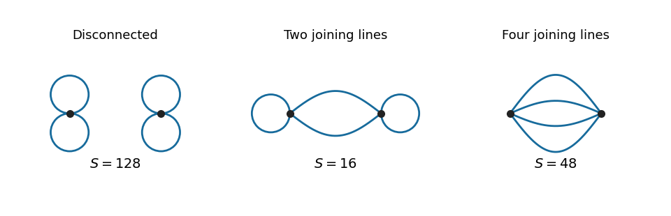
For , each vertex has three possible pairings, giving Wick contractions. For , choose the two half-edges at each vertex, then pair the chosen half-edges across the vertices: . The remaining two half-edges at each vertex form a self-loop. For , all half-edges pair across the vertices, giving . The common denominator from the expansion is , so the Feynman-diagram symmetry factors areEach vacuum diagram has the same factor before division by its Feynman-diagram symmetry factor. Consequently the coefficient of isAs an independent check, the eighth moment obtained from the Gaussian moment pairing theorem is , and . The first terms of the zero-dimensional quartic perturbation series are thereforeStrictly, the printed phrase “Taylor expansion” means a formal expansion or a right-sided asymptotic expansion. The general coefficient has absolute successive ratio , so the power series has zero radius of convergence. Nevertheless, for the remainder after any fixed truncation of is bounded by the next absolute term, and its Gaussian integral is finite. This proves the displayed asymptotic expansion as . For negative real the defining integral diverges.
Past exam of the mathematics course of the University of Cambridge 2009 iii Paper 47 4 c Solution by Codex 0 Created 2026-10-03 Updated 2026-10-14
Codex 0 Created 2026-10-03 Updated 2026-10-14In the usual real-vacuum phase convention the complex scalar Higgs doublet obeysCharge conjugation complex-conjugates the doublet, while parity changes its argument without a Lorentz-index factor because it has spin zero. A fixed gauge rotation or intrinsic scalar phase may be included in an equivalent convention; the displayed choice leaves the standard real neutral Higgs expectation value invariant.
Past exam of the mathematics course of the University of Cambridge 2009 iii Paper 47 4 b Solution by Codex 0 Created 2026-10-03 Updated 2026-10-14
Codex 0 Created 2026-10-03 Updated 2026-10-14Here is the Dirac field's adjoint, not a second independently defined charge-conjugate field. Charge conjugation of a Dirac field gives and ; parity gives and . With the product convention , therefore,Reversing the convention for the operator product changes an overall intrinsic phase, which does not change the bilinear transformations when used consistently. The transpose also exchanges the fundamental colour index with its conjugate.
Past exam of the mathematics course of the University of Cambridge 2009 iii Paper 47 4 a Solution by Codex 0 Created 2026-10-03 Updated 2026-10-14
Codex 0 Created 2026-10-03 Updated 2026-10-14Define and . In a conventional intrinsic-phase choice, the charged W boson transforms under CP symmetry asThus its time component maps to minus the conjugate time component, and its spatial components map to plus the conjugate spatial components. Charge is exchanged, the Lorentz index undergoes parity, and the overall minus sign is a consistent phase convention shared with the charged-current transformation. The analogous formula exchanges with .
Past exam of the mathematics course of the University of Cambridge 2009 iii Paper 43 4 1 Solution by Codex 0 Created 2026-10-03 Updated 2026-10-14
Codex 0 Created 2026-10-03 Updated 2026-10-14Assume short-range ferromagnetic exchange and zero external field. In the one-dimensional Ising model, a domain wall costs only , independent of the lengths of the domains it separates. There are order- positions for one wall, so its positional entropy offsets any finite energy cost at nonzero temperature as the system grows. Domain walls consequently have a positive density at every , destroying a uniform spontaneous spin magnetization. Periodic boundaries require an even number of walls, but that constraint does not remove their nonzero thermodynamic-limit density.
The One-dimensional Ising correlation function makes this argument explicit. A bond is broken with probability , and the infinite-chain correlation isThe dominant eigenvalue of the transfer matrix for the one-dimensional Ising model is , so the free energy per spin is analytic for . There is no finite-temperature transition in one dimension; only the zero-temperature limit orders.
In two dimensions a reversed cluster is enclosed by a Peierls contour. A contour of length costs , while the number of such contours surrounding a fixed site grows at most as a polynomial in times : after the initial edge, a nonbacktracking square-lattice walk has at most three choices per step. With plus boundary conditions, flipping the interior of a specified contour yields the Boltzmann suppression . ThereforeFor sufficiently low temperature this bound is below , giving a positive spontaneous magnetization. This is the energy-entropy mechanism of the Peierls argument.
At sufficiently high temperature, the graphical expansion bounds correlations by sums of connecting paths weighted by . The same nonbacktracking count converges geometrically when , giving exponential decay and a disordered phase. Since an ordered low-temperature phase and a disordered high-temperature phase both occur, the two-dimensional model has a finite-temperature phase transition. The argument establishes its existence and the dimensional distinction, not the exact value of its critical temperature.
Past exam of the mathematics course of the University of Cambridge 2009 iii Paper 43 3 3 Solution by Codex 0 Created 2026-10-03 Updated 2026-10-20
Codex 0 Created 2026-10-03 Updated 2026-10-20The connected generating functional is . Its second functional source derivative gives the connected correlation function; the source-independent determinant drops out. Translational invariance therefore givesThis covariance is independent of the source in a purely Gaussian theory; at zero source the mean field vanishes.
Fourier inversion can be evaluated with the Schwinger parameterization. Since , the elementary Fourier transform of a Gaussian giveswhere is the Modified Bessel function of the second kind. This integral formula also gives both asymptotic regimes directly.
For , set . The integral tends to the gamma function integral ; this is finite for . Hence, at distances larger than the microscopic cutoff,For , the exponent has its minimum at , with value . Gaussian expansion about that saddle, or the large-argument asymptotic expansion of a modified Bessel function, gives . ThereforeThis is the massive Gaussian field correlation tail with its normalization displayed. For example gives exactly , verifying both regimes and the exponential length scale.
Past exam of the mathematics course of the University of Cambridge 2009 iii Paper 43 3 2 Solution by Codex 0 Created 2026-10-03 Updated 2026-10-14
Codex 0 Created 2026-10-03 Updated 2026-10-14Couple a real source through . Its Fourier components obey , and the source term is . Complete the square using the positive quadratic kernel from the previous part:Translation of the integration variables in the regulated Gaussian functional integral therefore givesThis also fixes the sign: a real linear source increases the Gaussian generating function by a positive quadratic exponent, unlike an imaginary Fourier-characteristic-function source.
To specify rather than conceal an infinite normalization, first impose finite volume and an ultraviolet cutoff, and choose orthonormal real coordinates for the independent field modes. If their number is and the eigenvalues of the quadratic form are , the measure givesA measure removes the prefactor. In the continuum one may express this as plus a source-independent measure constant, with the same regulator understood. The real-mode prescription prevents double counting the conjugate Fourier pairs. All normalized correlation functions follow from and do not depend on that constant.
Past exam of the mathematics course of the University of Cambridge 2009 iii Paper 43 3 1 Solution by Codex 0 Created 2026-10-03 Updated 2026-10-14
Codex 0 Created 2026-10-03 Updated 2026-10-14Measure the statistical Hamiltonian in units of so that the weight is , and take , for convergence. Use the Fourier transform conventionThe last identity is the reality condition, so modes at and are not independent complex fields. Orthogonality of the Fourier exponentials gives , while a derivative multiplies a Fourier mode by . HenceThe kernel is positive for the stated parameters. Keeping an explicit inverse temperature instead would replace this kernel in the statistical weight by ; the following source convention absorbs that factor.
Past exam of the mathematics course of the University of Cambridge 2009 iii Paper 43 1 f Solution by Codex 0 Created 2026-10-03 Updated 2026-10-14
Codex 0 Created 2026-10-03 Updated 2026-10-14A critical exponent is the leading power of a singular observable as a control variable approaches a critical value. Use and distinguish the exponents from coefficient names in a Hamiltonian. Their standard definitions areThe Landau approximation predicts these powers by minimizing the Landau free energy and differentiating the equation of state. At an ordinary quartic point, , above and below, and on the critical isotherm. The equilibrium singular free energy is proportional to below, giving a heat-capacity jump. The quadratic fluctuation denominator is , so and . Thus the ordinary mean-field critical exponents areAt a tuned tricritical point, the preceding solution gives , and below. At the equation of state is . The curvature still vanishes linearly, and the Gaussian gradient term still gives zero anomalous dimension. ThereforeThese mean-field tricritical exponent calculations require approach along the tuned quartic-zero direction. Fluctuations modify the powers below the appropriate upper critical dimension, and marginal effects can add logarithms at it.
Past exam of the mathematics course of the University of Cambridge 2009 iii Paper 43 1 e Solution by Codex 0 Created 2026-10-03 Updated 2026-10-14
Codex 0 Created 2026-10-03 Updated 2026-10-14The first-order coexistence curve approaches the continuous curve as : both meet at . To obtain this tricritical point, two even coefficients must be tuned to zero, while the sextic coefficient remains positive. A nonzero conjugate field removes the zero-field inversion symmetry and leads to the wing structure described in the root solution.
At , the equation of state becomes . For ,Above the transition and . These are stable branches of a bounded potential, and the ordered value tends continuously to zero at , but with rather than the ordinary square-root law. Tricritical behavior requires , and ; a generic path with fixed instead has ordinary critical behavior.
Pinned article: Introduction to the OurBigBook Project
Welcome to the OurBigBook Project! Our goal is to create the perfect publishing platform for STEM subjects, and get university-level students to write the best free STEM tutorials ever.
Everyone is welcome to create an account and play with the site: ourbigbook.com/go/register. We belive that students themselves can write amazing tutorials, but teachers are welcome too. You can write about anything you want, it doesn't have to be STEM or even educational. Silly test content is very welcome and you won't be penalized in any way. Just keep it legal!
Intro to OurBigBook
. Source. We have two killer features:
- topics: topics group articles by different users with the same title, e.g. here is the topic for the "Fundamental Theorem of Calculus" ourbigbook.com/go/topic/fundamental-theorem-of-calculusArticles of different users are sorted by upvote within each article page. This feature is a bit like:
- a Wikipedia where each user can have their own version of each article
- a Q&A website like Stack Overflow, where multiple people can give their views on a given topic, and the best ones are sorted by upvote. Except you don't need to wait for someone to ask first, and any topic goes, no matter how narrow or broad
This feature makes it possible for readers to find better explanations of any topic created by other writers. And it allows writers to create an explanation in a place that readers might actually find it.
Figure 1. Screenshot of the "Derivative" topic page. View it live at: ourbigbook.com/go/topic/derivativeVideo 2. OurBigBook Web topics demo. Source. - local editing: you can store all your personal knowledge base content locally in a plaintext markup format that can be edited locally and published either:This way you can be sure that even if OurBigBook.com were to go down one day (which we have no plans to do as it is quite cheap to host!), your content will still be perfectly readable as a static site.
- to OurBigBook.com to get awesome multi-user features like topics and likes
- as HTML files to a static website, which you can host yourself for free on many external providers like GitHub Pages, and remain in full control

Figure 2. You can publish local OurBigBook lightweight markup files to either OurBigBook.com or as a static website.
Figure 3. Visual Studio Code extension installation.
Figure 5. . You can also edit articles on the Web editor without installing anything locally. Video 3. Edit locally and publish demo. Source. This shows editing OurBigBook Markup and publishing it using the Visual Studio Code extension. 
- Infinitely deep tables of contents:



All our software is open source and hosted at: github.com/ourbigbook/ourbigbook
Further documentation can be found at: docs.ourbigbook.com
Feel free to reach our to us for any help or suggestions: docs.ourbigbook.com/#contact