 Empirical distribution function

The empirical distribution function counts the fraction of observations at or below a threshold. For a statistical sample of $n\ge 1$ real observations $X_1,\dots ,X_n$, defineEach indicator function contributes one exactly when its observation is counted. Equivalently, $F_n(x)=P_n((-\infty ,x])$, where the empirical measure $P_n=n^{-1}{\sum }_i{\delta }_{X_i}$ assigns probability mass $1/n$ to each observation, including repeated observations.^[ref]

Choose the illustrative statistical sample $[1,1,2,4,6]$. Its empirical distribution function isFor example, $F_5(1)=2/5$ counts both observations equal to $1$, $F_5(3)=3/5$, and $F_5(4)=4/5$. There is no observation at $3$, so there is no jump there. The five observations produce only four distinct jump locations.

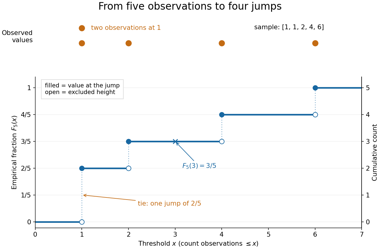
The convention $X_i\le x$ makes the empirical distribution function right-continuous: once a threshold reaches an observation, that observation remains counted immediately to its right. For a finite statistical sample, the count is constant from any $x$ up to the next larger observed value, proving right continuity. Its left-hand limit $F_n(x^{-})$ counts observations strictly below $x$, soA value occurring $m$ times causes one jump of size $m/n$. At $1$ the jump is $2/5$; at $2$, $4$, and $6$ each jump is $1/5$. All jumps sum to one. Thus the empirical distribution function is a nondecreasing step function with limits zero and one, and is itself a valid cumulative distribution function.

This turns many questions about data into simple cumulative distribution function operations. The observed fraction in $(a,b]$ is $F_n(b)-F_n(a)$: for $(1,4]$ it is $4/5-2/5=2/5$, counting $2$ and $4$ but excluding both $1$s. Including the left endpoint gives $F_n(4)-F_n(1^{-})=4/5$. A sample quantile reads the same staircase in reverse: the smallest threshold reaching $1/2$ is $2$. Unlike a histogram, this representation requires no choice of bins; its jumps retain every observation and its multiplicity.

The exact description of a finite statistical sample must be distinguished from a statistical model for how it was obtained. The empirical distribution function is defined for any finite list, with no independence assumption. Once the list is observed, its counts are fixed. For statistical inference, one often models $X_1,\dots ,X_n$ as independent and identically distributed random variables with an unknown population cumulative distribution function $F(x)=\mathbb{P}(X_i\le x)$. Then $F$ describes the sampling law, while $F_n$ varies across repeated statistical samples. The value $F_5(1)=0.4$ is an observed fraction and an estimate of $F(1)$; it does not establish that the population probability is $0.4$. Even when $F$ is continuous, every finite $F_n$ is discrete.

For any threshold $x$ fixed before sampling, the indicator functions are independent Bernoulli random variables with success probability $F(x)$. Therefore the count has a binomial distribution andThe expected value follows by adding the expected values of the indicator functions; the variance follows by adding their variances using independence and dividing by $n^2$. Thus $F_n(x)$ is an unbiased estimator of $F(x)$ at a fixed threshold. Controlling the error at every threshold at once requires more than a fixed-threshold calculation: the DKW inequality supplies such control, and the Glivenko-Cantelli theorem describes its uniform convergence almost surely as $n$ grows.

Comparing $F_n$ with a proposed cumulative distribution function also motivates goodness-of-fit tests, including the Kolmogorov-Smirnov test, the Anderson–Darling test, and the Cramér–von Mises criterion. A standard Kolmogorov-Smirnov test calibration assumes a fully specified continuous population law; fitting its statistical parameters from the same statistical sample changes that calibration.^[ref]