
For a stable input with path action , a workload x requires some interval of length t with average input near . Jensen inequality bounds its cost below by ; taking the supremum workload and then the infimum over t yields the displayed lower bound. Constant-rate burst paths give the matching upper bound. At zero the typical-rate path has zero cost; negative workloads have infinite rate. If no finite-cost rate exceeds C, every positive workload has infinite rate.
Stationary workload supremum 2026-10-14
For independent and identically distributed arrivals with finite mean below service , the strong law of large numbers makes the net cumulative input tend to minus infinity, so the supremum is finite almost surely. Applying the same formula to the past input gives a stationary solution of the Lindley recursion. This representation turns queue workload overflow into an event involving some lookback horizon.
Word metric balls in the integer lattice 2026-10-14
The additive group gives a useful way to see what a word metric measures. Let and , and choose the four-move generating set of a group . Its Cayley graph is the square lattice. Each move changes exactly one coordinate by one, so the word length is the L1 norm, and the word metric is Manhattan distance:At least this many moves are necessary, and moving horizontally then vertically attains the bound. Bridson gives this square lattice as a basic Cayley graph example.[ref]
Now allow all eight neighbouring lattice points as moves:Each coordinate changes by at most one per move. Use diagonal moves until the smaller displacement is exhausted, then use axis moves: the resulting word length is the maximum norm, and the word metric is Chebyshev distance. From to , an -route has five steps, while the -route has three.
The closed word metric balls consist of lattice points inside a diamond for , and inside an axis-aligned square for . For every nonnegative integer radius ,The diamond has lattice points at word length ; the square has choices for each coordinate. At radius three the counts are and . These are discrete closed balls for Manhattan distance and Chebyshev distance; an Euclidean distance bound would instead select lattice points inside a Euclidean disk.
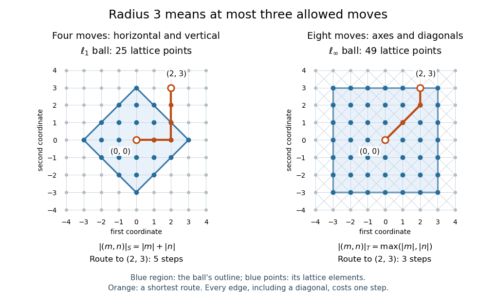
Radius-three word metric balls in the integer lattice: a diamond with 25 points and a square with 49 points, with routes to
. Details. Sen spinor connection 2026-10-14
Restrict the spacetime spin connection to a spacelike hypersurface. With future unit normal and convention , it differs from the intrinsic spin connection by the displayed extrinsic curvature term. Its spatial Dirac operator is the operator in the Witten spinor equation; replacing it by the intrinsic operator would omit the ADM momentum contribution.
Elliptic existence of a Witten spinor 2026-10-14
On complete smooth asymptotically flat spin initial data without inner boundary, satisfying the Einstein constraints and the dominant energy condition, the Witten spinor equation admits a spinor approaching each prescribed asymptotic constant, under the standard weighted decay assumptions. The integrated Witten-Nester identity gives a coercive estimate and excludes a decaying homogeneous kernel. Weighted elliptic solvability then supplies the desired correction to a spinor extended from infinity. Positivity of the boundary integral is a conditional identity until this analytic existence step is supplied; see the rigorous analytic proof.
Inward transport by an angular-momentum-enhanced disk wind Created 2026-10-14 Updated 2026-11-05
For zero viscosity, and constant , set . On intervals where f>0, the wind-loaded Keplerian disk evolution equation becomes . Multiplication by and the displayed travel-time coordinate reduce it to constant-speed advection. Its profile is and its characteristics move inward with . The weight accounts for mass loss as well as radial compression.
Skumanich rotation law Created 2026-10-14 Updated 2026-11-05
If the moment of inertia I changes slowly and wind-driven magnetic braking of a solar-type star has torque , then . At sufficiently late times within this unsaturated approximation, rotation scales as . This empirical main-sequence trend is not a universal law for saturated rapid rotators, changing stellar structure or every magnetic geometry.
Wiener theorem 2026-10-14
There exists a probability measure on under which the coordinate process is standard Brownian motion, and its distribution there is unique. Construct consistent centered Gaussian finite-dimensional laws with covariance and use the Kolmogorov extension theorem. The fourth increment moment supplies a continuous modification by the Kolmogorov continuity theorem. Its independent increments and normal increment distributions are unchanged. Uniqueness follows because coordinate evaluations at rational times generate the Borel sigma-algebra of continuous-path space.
Mixed Dirichlet-Neumann half-plane diffraction Created 2026-10-14 Updated 2026-10-31
For a scalar wave above a line with a Dirichlet half and a Neumann half, the boundary transform factors into and . For , the limiting absorption principle puts below and above the inversion contour. With Dirichlet conditions on the negative half-line and incident tangential wavenumber , pole subtraction gives the diffracted trace . Its large-transform decay gives a bounded field with a square-root edge trace. The normal derivative has an inverse-square-root singularity on the Dirichlet half; it is identically zero on the Neumann half.
Whitehead square 2026-10-14
The Whitehead square of a class is . For the identity class of an even-dimensional sphere, the Hopf invariant is two with the standard product-cell orientation: folding the two sphere summands makes the middle cohomology class of the mapping cone pull back to on , and . For odd , graded symmetry makes the square two-torsion, hence rationally zero.
Continuous-time Gaussian white noise 2026-10-14
Continuous-time Gaussian white noise is a random distribution rather than an ordinary finite-variance function at every time. Integrating it against deterministic kernels gives Gaussian random variables with covariance . For independent isotropic components, a three-dimensional dot covariance has amplitude . An ordinary rapidly decaying force covariance approximates this model only above its correlation time.
Discrete Gaussian white noise Created 2026-10-14 Updated 2026-11-05
Discrete Gaussian white noise is a jointly Gaussian sequence with expected value zero and covariance at lag zero and zero at other lags. Joint normality makes the components independent. This is a sequence of ordinary random variables, unlike the generalized continuous-time white-noise process.
Higman's lemma 2026-10-14
If is a well-quasi-ordering, its finite words form a well-quasi-ordering under subsequence embedding with coordinatewise increase of letters. A minimal bad sequence proof removes the last letter of selected words whose last letters form a nondecreasing subsequence, then contradicts minimality. The result implies finite-subset lifting of a well-quasi-order under Hoare domination preorder.
Better-quasi-ordering 2026-10-14
A quasi-order is better-quasi-ordered if every array into it from every barrier in better-quasi-order theory is good: some barrier members satisfy . Singleton barriers recover the usual infinite-sequence condition for a well-quasi-ordering. The stronger condition is useful for infinitary closure operations for which well-quasi-ordering alone fails. Equivalently one may use continuous maps from infinite subsets of an infinite subset of the natural numbers, with the discrete topology on the range, and compare with .
A finite Cartesian product of well-quasi-orderings is well-quasi-ordered in the componentwise order. Every infinite sequence in one well-quasi-order has an infinite nondecreasing subsequence: colour pairs by whether they are ordered, apply Ramsey's theorem, and exclude an all-bad subsequence. Restrict successively to such a subsequence in each coordinate. The same argument, or the infinite pigeonhole principle, proves closure under finite disjoint unions with no cross-component comparisons.
Perfect subsequence lemma 2026-10-14
Every infinite sequence in a well-quasi-ordering has an infinite subsequence all of whose earlier terms precede its later terms. Some term must have infinitely many later terms above it: otherwise choose each new index outside the finitely many upper-cone index sets of the terms already chosen, producing a bad sequence. Apply the same observation successively inside the infinite upper-cone subsequence. Each restriction preserves all earlier inequalities, proving the assertion.
Regular locale 2026-10-14
A locale is regular when every open is the join of opens well inside it. This expresses regularity without reference to points.
Well-formed weighted projective space 2026-10-14
A weighted projective space with positive integer weights is well-formed when the greatest common divisor of the weights with any one weight omitted is one. The quotient toric lattice is free and the images of the coordinate vectors are primitive toric rays. Its fan contains the cones on all proper subsets of these rays.
Weighted mean minimizes squared deviations 2026-10-14
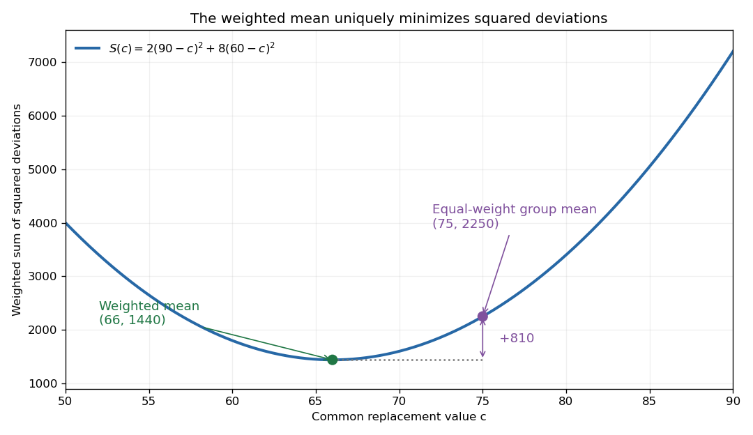
For a finite list of real numbers and nonnegative weights of positive total , the weighted mean uniquely minimizes the weighted sum of squared deviationsExpanding around and using givesEvery displacement from the weighted mean increases the objective. This is the simplest one-parameter weighted least squares problem: represent all entries by one common value.


Combining means of groups Created 2026-10-14 Updated 2026-10-25
Suppose disjoint nonempty groups have sizes and arithmetic means . The arithmetic mean of all observations isEach group contributes the sum ; add those totals before dividing by the overall count. This is exactly a weighted mean of group means with weights equal to group sizes. [ref]
Take a synthetic example with two observations equal to and eight equal to . The two group means are and , and the combined mean is . Giving the two groups equal weights instead produces , which summarizes the two group means with equal influence. To summarize all ten individuals with equal influence, use their group counts.
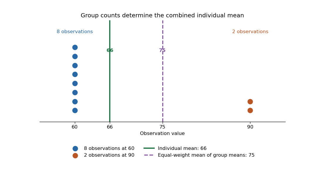

The group means and counts determine the combined arithmetic mean, but do not generally determine the combined variance. Variation within the groups is additional information.
There are unlisted articles, also show them or only show them.