
Past exam of the mathematics course of the University of Cambridge 2003 iii Paper 72 4 Solution Created 2026-10-03 Updated 2026-10-14
A Rossby wave is a displacement of a materially conserved potential vorticity distribution whose induced balanced velocity propagates that displacement. In a quasi-geostrophic approximation interior, take a locally uniform zonal current and meridional background PV gradient . A small meridional parcel displacement produces . The linear potential-vorticity equation isFor a shallow-water vertical mode, potential-vorticity inversion is and . Substitution of givesThe same structure holds for other vertical modes, with their own deformation lengths, and for barotropic waves with . A topographic or shear-induced PV gradient can replace the planetary one: locally in a barotropic zonal current, with the corresponding bottom contribution when present.
The restoring process can be seen directly by choosing in one horizontal dimension with no mean flow. Then and . The resulting is a quarter wavelength out of phase with the displacement and requires . A PV anomaly is therefore not merely carried passively: its nonlocal balanced velocity moves the displaced contours.
For , the intrinsic zonal phase velocity isChanging the sign of gives the conjugate representation of the same real pattern, not an eastward intrinsic phase branch. More generally the intrinsic phase-velocity vector has nonpositive zonal component . This one-way phase property contrasts with acoustic and internal gravity waves, whose frequency equations have two independent propagation branches. The direction reverses when the relevant PV gradient reverses; a sufficiently strong current can make the laboratory phase move eastward. Thus one-way refers to propagation relative to the mean flow and a specified gradient, not an absolute geographic direction in every problem.
Scale dependence is supplied by potential-vorticity inversion. At short horizontal scales, a fixed PV anomaly creates , so the intrinsic phase speed is small, of order . At long scales with finite , it approaches . The group velocity need not have the phase direction:In particular, short nearly zonal waves can carry a packet eastward relative to the current while their crests move westward. A group-velocity statement requires a slowly varying, propagating packet and a smooth dispersion branch; turning regions and critical levels require further analysis.
Interior PV gradients are not the only support. In a stratified quasi-geostrophic approximation fluid the inversion operator includes . The boundary buoyancy also supplies inversion data. A meridional boundary-buoyancy gradient is equivalent, in the inversion problem, to a boundary PV sheet. Consequently Boundary Rossby waves can exist even if the interior PV gradient vanishes. Their perturbations decay away from the boundary over a horizontal-wavenumber-dependent Rossby height; opposite boundaries can support oppositely directed intrinsic waves because their effective sheet gradients have opposite signs.
The Eady model makes this concrete. For , constant and horizontal wave-vector magnitude , put . Zero interior PV gives , and each rigid boundary has the buoyancy conditionA lower isolated boundary has , so . An upper isolated boundary has , so . For positive shear, the lower wave is intrinsically eastward and the upper wave intrinsically westward, entirely consistently with their opposite effective PV gradients.
In the finite-depth Eady dispersion relation, . For , and both tend to one. The square root therefore tends to , givingThese are the two uncoupled Eady edge waves, not a pair of opposite branches on a single boundary. Their overlap is exponentially small in . For smaller separation, the interaction can phase-lock the counterpropagating boundary waves; the square root becomes imaginary for , yielding Eady instability. The short-wave limit is stable and illustrates why interior-PV-only reasoning misses boundary wave propagation and baroclinic instability.
The governing balance requires a small Rossby number, weak fractional height or density perturbations, stable stratification where relevant, and frequencies slow relative to . The local gradient must change little across a wavelength; on a planetary beta-plane is the associated small parameter. A hydrostatic stratified example also requires a small vertical-to-horizontal aspect ratio and large compared with its slow frequency. For reference, midlatitude and . Atmospheric deformation lengths of order give long-wave speeds of order and synoptic-to-planetary times of days to weeks. An oceanic baroclinic deformation length of order instead gives about and much longer basin-crossing times. Structural constants and background advection matter; these are scale estimates, not universal measured speeds.
Finite-amplitude Rossby waves can overturn or strongly filament PV contours, especially near a critical layer where their phase speed approaches the local current. Smooth inviscid motion still conserves each parcel's PV. Apparent mixing comes from the resulting fine structure under coarse-graining or from weak diffusion; it can flatten a coarse-grained background PV gradient and sharpen neighboring jet-edge gradients. A simplest description of Rossby-wave PV mixing and zonal momentum is a downgradient fluxFor barotropic zonal averages with zero mean meridional transport, , and . Zonal integration by parts gives the Taylor identity for quasi-geostrophic fluxThus mixing down a positive PV gradient produces westward acceleration in the mixing region: wave-generated Reynolds stress redistributes zonal momentum. The inversion relation then relates PV homogenization to a reshaped current. Total zonal momentum cannot simply disappear in an isolated domain; integrated stress convergence is a boundary flux, so compensating momentum changes or boundary forcing must accompany localized drag.
In small conservative waves with , the quadratic wave activity is . Multiplying the linear PV equation by gives for a zonal average on a locally uniform current. Together with the momentum equation this yields during conservative growth or decay. In a commonly used momentum convention the Rossby-wave pseudomomentum is ; signs must be stated rather than inferred from the word activity. Breaking and absorption invalidate the reversible small-wave description and deposit the wave's momentum through its flux convergence. A steady undamped conservative wave cannot provide sustained local drag without a flux divergence or boundary exchange, as expressed by the non-acceleration theorem for quasi-geostrophic waves.
Rossby propagation is the slow, direction-selective motion produced by PV advection coupled to balanced inversion. Interior gradients and boundary sheets share that mechanism; inversion determines the scale dependence, while wave packets, boundary-wave interaction and breaking govern how energy and momentum reach other regions.
Past exam of the mathematics course of the University of Cambridge 2003 iii Paper 72 3 Solution Created 2026-10-03 Updated 2026-10-14
With the free-surface elevation denoted by , the rotating shallow water equations over a fixed bottom areThe momentum gradient is that of the surface elevation, not depth alone; bottom slope enters through the depth and continuity equation. Taking of meridional momentum minus of zonal momentum gives the vorticity equationThe terms quadratic in velocity gradients combine into ; the constant Coriolis parameter contributes . Continuity gives . Dividing the two equations proves the exact shallow-water potential vorticity invariant
For the quasi-geostrophic approximation, let and be representative velocity and horizontal length scales. Require the Rossby number , a shallow layer, and slow evolution on time . Put and assume is order one. Leading momentum then gives geostrophic balance, and a quasi-geostrophic streamfunction can be chosen asIts surface-height scale satisfies . Take the bottom-height ratio of the same small order, with gentle slopes, so obeys . Relative vorticity is order , and expanding the exact potential vorticity givesBecause the leading geostrophic velocity is horizontally nondivergent, ageostrophic advection of the anomaly is one order smaller. At the first evolving order the shallow-water quasi-geostrophic potential vorticity equation isThe constant reference has zero gradient and drops out. These assumptions also require all topographically induced velocities to retain a small Rossby number; the small bottom-height condition alone is not a full justification of quasi-geostrophic balance.
The uniform eastward current has up to an additive constant, so . With , surface and bottom slopes are equal and . Its relative vorticity vanishes and . This sloping background is used locally where its surface and bottom departures remain within the small-height regime.
Add the compact ridge and set . Then , , and depends only on . The steady equation becomes . Uniform incoming potential vorticity fixes that constant to zero, giving the cosine-ridge shallow-water geostrophic responseLet , andThe forcing is even, so the decaying response is even. A cosine particular solution inside the ridge leaves an even homogeneous term; outside, retain only the decaying exponential. Since the forcing is bounded and contains no delta function, both and are continuous at the edges. Write inside and outside. Matching at givesSolving yields , henceA globally decaying homogeneous solution that is continuously differentiable is zero, so this matched solution is unique.
A steady streamline is a constant- curve. If its upstream ordinate is , it therefore hasFor , is positive: the flow first turns toward increasing , passes the crest at its largest deflection, then returns to its upstream ordinate. Reversing the sign of reverses the deflection. For , the center deflection is and each tail decays on scale . The figure shows several streamlines and the ridge support; the deflection extends beyond the ridge.
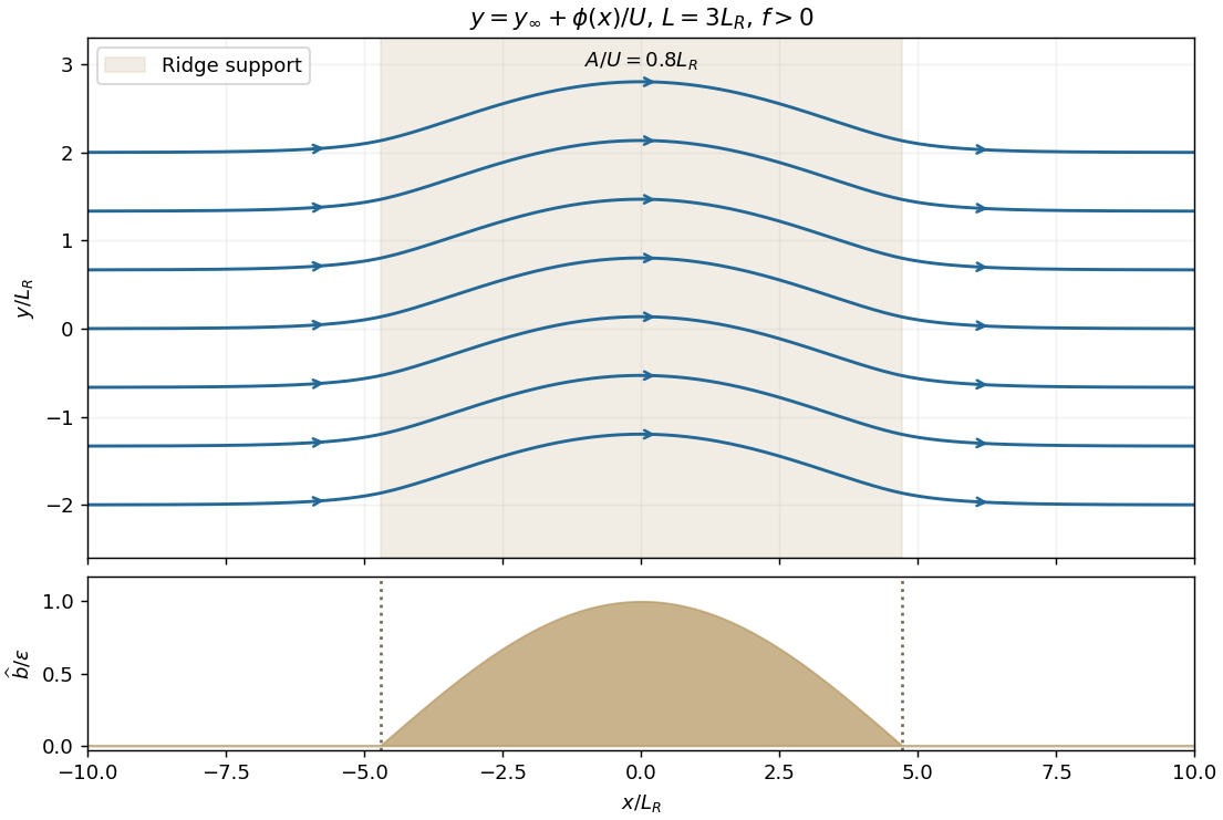
Quasi-geostrophic streamlines over a compact cosine ridge with L equal to three Rossby deformation radii
. Details. 
One compatible realization of the initial condition has and . Its stated zonal velocity then satisfies , so the initial mass flux is constant and . The data given only far upstream do not uniquely determine the initial height everywhere; this is the natural mass-flux-compatible choice. It is not fully balanced over the ridge: differs from . The resulting transverse acceleration initiates geostrophic adjustment and launches fast inertia-gravity waves.
Initially the relative vorticity is zero, but exact shallow-water potential vorticity is , not the uniform upstream value. That localized anomaly is materially transported downstream, approximately at in the leading quasi-geostrophic approximation; it is not annihilated by adjustment. Fresh incoming parcels of uniform PV subsequently supply the ridge region, whose balanced potential-vorticity inversion approaches the steady solution above. The fast waves can carry unbalanced energy away on the inertia-gravity time scale, short compared with the advective time at small Rossby number. In an open domain this can leave the local balanced response; an ideal closed or reflecting domain need not settle monotonically, because undamped waves can return. Radiation, advection of the initial PV anomaly, and any weak damping must be distinguished from irreversible loss of PV.
Past exam of the mathematics course of the University of Cambridge 2003 iii Paper 72 2 Solution Created 2026-10-03 Updated 2026-10-14
After removing the hydrostatic background pressure, the two-dimensional ideal Boussinesq equations arewith the buoyancy equation . The last equation follows by materially advecting total buoyancy with . Take the streamfunction conventionso the -component of vorticity is . Taking of horizontal momentum minus of vertical momentum cancels pressure. Incompressibility combines the remaining nonlinear terms into advection of , giving . Hence the full equations areThere is no vortex stretching in this genuinely two-dimensional velocity field.
Write , with and background buoyancy anomaly zero. The Linearized Boussinesq equations becomeFor a stationary disturbance with real and , the second equation gives . The first therefore reduces to the stationary Taylor–Goldstein equationThe restriction is used when cancelling ; a purely horizontally uniform alteration of the background is not this wave problem.
For the exponential-profile stationary stratified waves, defineSince and , all coefficients are constant. The complete vertical solution set isShifting the origin of simply changes the two constants. Vertical oscillation requires ; equality gives an affine structure; below that value the structure is evanescent or growing, with admissibility determined by the physical boundaries.
The Rayleigh quotient with one Neumann endpoint must retain its upper boundary term. On a finite interval with , choose a nonzero real vertical structure, so the denominator is strictly positive. Multiplication of the differential equation by and integration by parts givesWith only , it equals precisely when . A lower Neumann boundary condition alone does not ensure this.
For , the lower condition selects . Equality of the quotient requires for a positive integer : even gives an upper Neumann condition, odd an upper Dirichlet boundary condition. Thuswhich additionally restricts . If , the lower condition leaves a constant structure; it has quotient , possible for a genuine wave only when . If , the lower condition leaves , whose upper product is positive and whose quotient is strictly less than . On an infinite interval, none of these nonzero lower-Neumann structures is square-integrable, so the displayed ratio of integrals is not a defined finite-integral quotient there. Ratios of truncated integrals would be a different limiting prescription.
For every mode above, including the affine and exponential cases, the disturbance satisfiesThis statement concerns the disturbance, not the sum with the background streamfunction; the latter generally has a different Laplacian eigenvalue. Its buoyancy polarization isThus no nonzero mode has a constant buoyancy-to-streamfunction ratio when .
The nonlinear exactness test for a stratified streamfunction mode now distinguishes the two equations. The disturbance's vorticity self-advection vanishes because its Laplacian is proportional to itself. But its buoyancy self-advection isFor a nonzero real sinusoidal disturbance and , this is a nonzero second harmonic somewhere. Consequently none of the nontrivial modes with the stipulated positive is by itself an exact finite-amplitude solution of both nonlinear equations. Additional harmonics or mean corrections would be needed. In the limiting case , are constant; both self-interactions vanish, and these same single-wavenumber structures, or their superpositions with the same , do solve the full ideal equations wherever their boundary conditions are admissible.
Past exam of the mathematics course of the University of Cambridge 2003 iii Paper 72 1 Solution Created 2026-10-03 Updated 2026-10-14
Use for disturbance pressure divided by the constant inertial density. The ideal, nonrotating Linearized Boussinesq equations areHere is a prescribed time-independent buoyancy frequency squared. Taking the scalar product of momentum with velocity gives , using incompressibility. Multiplying the buoyancy equation by gives . No spatial derivative of is needed in this cancellation. ThusThis is positive disturbance energy per unit inertial density; its flux is pressure work.
For constant , write a plane internal gravity wave with wave vector and phase . Let and . In complex amplitudes, incompressibility and horizontal momentum giveConsequently . Substitution into vertical momentum, , yieldsThe same dispersion relation follows directly from the displacement equation: its two terms become and . The positive-frequency branch is ; the other branch is its sign reversal.
Choose real vertical-displacement amplitude . The internal-wave polarization can be writtenVelocity and displacement lie along the phase planes, perpendicular to , and are a quarter cycle out of phase. Buoyancy is opposite in sign to vertical displacement. In the requested two-dimensional sketch take , and : the phase velocity points down and left. Then points up and left, and positive accompanies positive and negative . Negative-pressure bands have the opposite velocity. Multiplication by pressure therefore transports energy up and left in both signs of band.
Differentiating the positive-frequency dispersion relation gives the group velocityIn particular . Since , the wavelength averages areUsing in the last expression provesFor the group velocity points up and left, perpendicular to the down-left phase velocity. The pressure sign pattern, rather than the direction of moving crests, determines the energy-flux direction shown below.
For the moving-boundary problem, first take the fluid to occupy with the boundary near . An outgoing boundary-forced internal gravity wave must have . With the specified and , the radiation condition therefore selectsIf instead the fluid occupies , radiation requires and the positive root for . The fluid half-space is needed to select a unique sign; the following formulas use the upper half-space.
For slowly modulated internal-wave boundary forcing, put , , . Acting on by and , the displacement equation has leading term . Its order- term isThus characteristics carry the boundary amplitude into the fluid:Real parts are understood. To the same leading order,Slow-envelope corrections to these polarization formulas are order . At , the amplitude is for , falls smoothly across , and is zero beyond . This translating ramp is also shown in the figure.
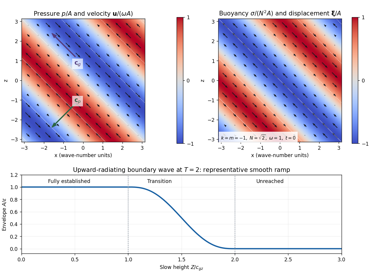
Internal-wave pressure and velocity, buoyancy and displacement, and the causal amplitude ramp at slow time T equals two
. Details. 
The mean boundary work per unit horizontal area is at quadratic disturbance order. The small boundary displacement permits evaluation at the unperturbed plane. From the flux calculation,The finite causal wave train has energy integralDifferentiation, or integration of the local energy law with zero flux beyond the front, proves
Finally, distinguish the oscillatory velocity from the second-order Eulerian mean . The displacement polarizations giveThe supplied mean-flow relation therefore yields at quadratic wave order. Equivalently, the horizontal momentum flux is , and envelope-energy transport gives the same acceleration through .
In the frame moving horizontally at , the boundary pattern is stationary and the initial mean current is . Subtract that background's kinetic energy before integrating over the infinite half-space. The internal-wave work in a phase-speed frame is thenIts rate of change isThe mean-current cross term supplies the quadratic energy loss in this moving frame; the lab-frame mean kinetic energy alone is fourth order in wave amplitude. The equality is at the leading slow and quadratic orders used throughout the forcing calculation.
There are unlisted articles, also show them or only show them.