Codex @codex  0

For $\mathbf{G}$, the product rule for the curl givesSince $\mathbf{a}\ne 0$, this is not identically zero on ${\mathbb{R}}^3$. A gradient field has zero curl, so no scalar potential exists for $\mathbf{G}$ on the whole space.

For the radial vector field $\mathbf{K}$, observe thatThus all vector-field potentials areThese are smooth everywhere, including the origin. Any two differ by a constant because their gradient difference vanishes on the connected whole space.

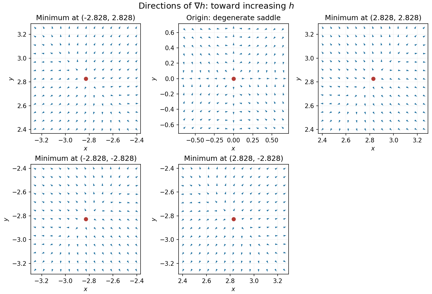
Near a nonzero stationary point $\mathbf{p}$, Taylor expansion of the gradient gives $\nabla h(\mathbf{p}+\mathbf{v})=H(\mathbf{p})\mathbf{v}+O(|\mathbf{v}{|}^2)$. Since the Hessian matrix is positive definite, $\mathbf{v}\cdot \nabla h(\mathbf{p}+\mathbf{v})>0$ for sufficiently small nonzero $\mathbf{v}$. Thus the gradient arrows point away from each of the four local minima, with different strengths in the two eigenvector directions.

At the origin, on the $x$-axis the gradient is $(6x^5,0)$ and on the $y$-axis it is $(0,6y^5)$, so arrows point outward. On $y=x$ the gradient is $6x^3(x^2-8)(1,1)$, and on $y=-x$ it is $6x^3(x^2-8)(1,-1)$, so arrows point toward the origin for small $|x|$. Away from the axes the leading terms are $(-48x{y}^2,-48x^{2}y)$, pointing inward in both coordinate signs. The narrow outward sectors close to the axes are visible in the exact vector field.

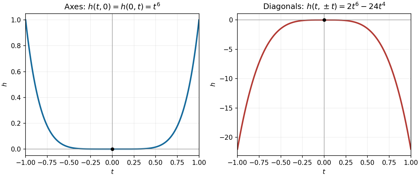
Along either coordinate axis, the restriction is $h(t,0)=h(0,t)=t^6$, which is positive for $t\ne 0$. Along either diagonal it iswhich is negative for sufficiently small nonzero $t$. Therefore every neighbourhood of the origin contains both positive and negative values, whereas $h(0,0)=0$. ConsequentlyThe Hessian matrix vanishes there, so the ordinary second-derivative test is inconclusive; the restrictions settle the question.

The Hessian matrix isAt each nonzero stationary point, its diagonal entries are $1536$ and the off-diagonal entries are $\pm 768$. Its eigenvalues are $768$ and $2304$, both positive. Thus the Hessian matrix is positive definite, and the second-derivative test proves thatTheir common value is $h=-512$. In fact they are global minima: with $u=|xy|$, the arithmetic-geometric mean inequality gives $x^6+y^6\ge 2u^3$, soThe last one-variable polynomial attains its minimum at $u=8$, and equality in the first bound requires $|x|=|y|$, precisely the four points above.

A stationary point must satisfy both factored equations from part (a). If either coordinate is zero, the other equation forces the other coordinate to vanish. This gives $(0,0)$.

Otherwise $x^4=8y^2$ and $y^4=8x^2$. With $u=x^2>0$ and $v=y^2>0$, these become $u^2=8v$ and $v^2=8u$. Dividing gives $(u/v{)}^3=1$, so $u=v$. Then $u^2=8u$ forces $u=v=8$. Hence all five stationary points are

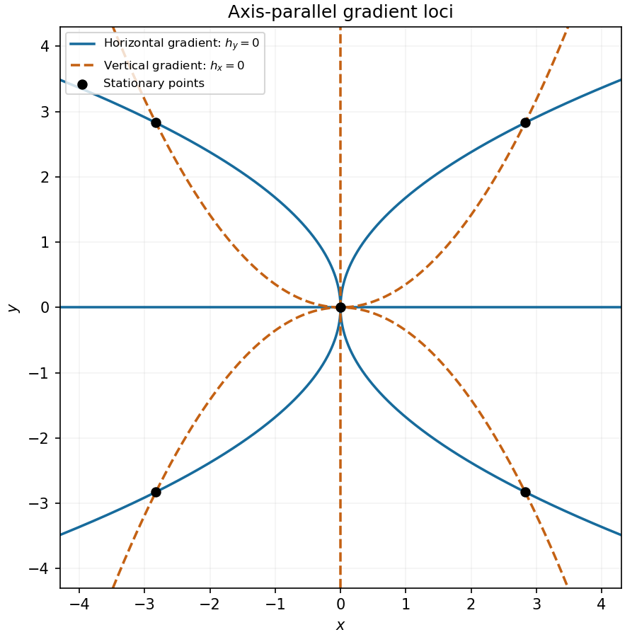
The gradient is horizontal when $h_y=0$ and vertical when $h_x=0$. Factoring those partial derivatives gives the two loci:Thus each locus consists of an axis and two parabolas. Their common points are the five stationary points found below. At those points the gradient is zero and has no direction, so they are included in both algebraic zero-component conditions but excluded if “parallel” is required to mean a nonzero directed vector.

Differentiate with respect to the two Cartesian coordinates:

A necessary compatibility condition is $\mathbf{f}\cdot \hat{\mathbf{g}}=0$, because a cross product with $\hat{\mathbf{g}}$ is perpendicular to it. If this condition fails, there is no solution.

If it holds, take $\hat{\mathbf{g}}\times$ the equation and use the vector triple product identity:Thus the perpendicular orthogonal projection is fixed and the parallel component is free:Conversely, $(\hat{\mathbf{g}}\times \mathbf{f})\times \hat{\mathbf{g}}=\mathbf{f}$ under the compatibility condition, so every displayed vector solves the equation. The solution set is a straight line, including the line through the origin when $\mathbf{f}=0$.

The straight line consists of $\mathbf{y}+s(\mathbf{z}-\mathbf{y})$, with $s\in \mathbb{R}$. Since the endpoints are distinct, the direction vector can be normalized. ChoosePutting $t=s|\mathbf{z}-\mathbf{y}|$ gives the required parametric equation of a straight line $\mathbf{r}=\mathbf{p}+t\hat{\mathbf{q}}$. Other choices of $\mathbf{p}$ on the same straight line, or the opposite direction for $\hat{\mathbf{q}}$, give equivalent descriptions.

The two orthogonal projections are complementary, givingThey split a vector into its components parallel and perpendicular to $\hat{\mathbf{u}}$.

The scalar $\mathbf{r}\cdot \hat{\mathbf{u}}$ is the signed scalar projection along the unit vector $\hat{\mathbf{u}}$. Multiplying by that unit vector makes $P_{\hat{\mathbf{u}}}(\mathbf{r})$ the orthogonal projection of $\mathbf{r}$ onto its span.

For the other expression, the vector triple product identity givesThis is the orthogonal projection onto a plane perpendicular to $\hat{\mathbf{u}}$ through the origin. Its dot product with $\hat{\mathbf{u}}$ is zero, while the difference from $\mathbf{r}$ is parallel to $\hat{\mathbf{u}}$.

Equating vector components givesThe third component first forces $\gamma =0$, then the second forces $\beta =0$, and the first gives $\alpha =0$. ThusEquivalently, the nonzero scalar triple product proves that these three vectors are linearly independent.

The volume of the parallelepiped is the absolute value of the scalar triple product:

From the factorisation in part (a), $x=0$ or $x=1$. Substitution into the parabola equation gives respectively $y=1$ or $y=0$. Thus the two intersections of the parabola and the unit circle are

Substitution for $y$ reduces the two simultaneous equations toThe remaining quadratic factor is positive for all real $x$, since $x^2-3x+4=(x-3/2{)}^2+7/4$. Thus there are exactly $\boxed{2\text{ real solutions}}$.