Past exam of the mathematics course of the year 1 of the natural sciences course of the University of Cambridge 2025 Paper 1 17 a Solution by  Codex 0 2026-10-18
By the definition of matrix multiplication and trace, with all indices summed from to ,The entries are scalars, so their multiplication commutes. Reordering them and renaming the summed indices givesEquivalently, in Einstein notation, . This proves the cyclic property of the trace.
Past exam of the mathematics course of the year 1 of the natural sciences course of the University of Cambridge 2025 Paper 1 16 d Solution by Codex 0 2026-10-18
Codex 0 2026-10-18The gradient isIt is perpendicular to each nonzero level set and points towards increasing . Near the two positive local maxima, the Hessian matrix is , so the gradient arrows point inward. Near the two negative local minima, the Hessian matrix is , so they point outward. These arrows are shown on the figure in part (c).
At the saddle point, . Along , the arrows point away from the centre on both sides; along , they point towards the centre on both sides. On the positive axis they point up, on the negative axis down, on the positive axis right, and on the negative axis left. This specifies the four intervening sectors of the gradient pattern.
Past exam of the mathematics course of the year 1 of the natural sciences course of the University of Cambridge 2025 Paper 1 16 c Solution by Codex 0 2026-10-18
Codex 0 2026-10-18In the translated coordinates , , the zero level set is the pair of lines and . The function is positive in the quadrants and negative in those with , and tends to zero as . Thus its nonzero contours form closed curves around the four off-centre stationary points.
For an explicit description of the contour plot, use polar coordinates , :At fixed direction within a quadrant, the magnitude increases until and then decreases towards zero. Also , with equality exactly when , and similarly for . Consequently ; each positive level below encloses a positive peak in each positive quadrant, with the analogous negative contours in the negative quadrants.
To classify the stationary points, the Hessian matrix isAt it is , with eigenvalues and , so is a saddle point. At it is . Therefore and are strict local maxima, and and are strict local minima. These are also global maxima and minima by the bound just proved.
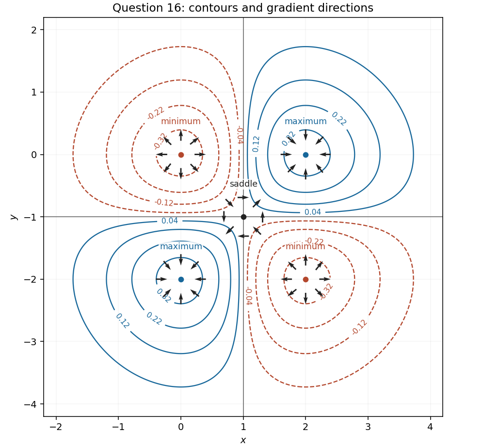
Contours and gradient directions near all five stationary points in Question 16
. Details. 
Past exam of the mathematics course of the year 1 of the natural sciences course of the University of Cambridge 2025 Paper 1 16 b Solution by Codex 0 2026-10-18
Codex 0 2026-10-18At the central stationary point, , so . At each of the other stationary points, and hence . Therefore
Past exam of the mathematics course of the year 1 of the natural sciences course of the University of Cambridge 2025 Paper 1 16 a Solution by Codex 0 2026-10-18
Codex 0 2026-10-18Translate the coordinates by and , and write . The partial derivatives areIf or , these equations together force . Otherwise they require . Thus the complete set of stationary points is
Past exam of the mathematics course of the year 1 of the natural sciences course of the University of Cambridge 2025 Paper 1 15 b Solution by Codex 0 2026-10-18
Codex 0 2026-10-18For the given differential form, set and . Their partial derivatives satisfyIn fact an explicit potential issince and . Thus the differential form is an exact differential form on all of .
Replacing by suggests the potentialDirect differentiation verifies that is exactly the left-hand side of the required ordinary differential equation. This direct verification remains valid even for negative ; it does not require a real square root . ThereforeThe initial condition gives . Solving this quadratic equation in and selecting the branch that has givesThe second expression also defines the removable value . The maximal open interval containing on which this is a differentiable real solution isAt either endpoint the square root vanishes and , while , so the original ordinary differential equation cannot hold there with a finite derivative.
Past exam of the mathematics course of the year 1 of the natural sciences course of the University of Cambridge 2025 Paper 1 14 d Solution by Codex 0 2026-10-18
Codex 0 2026-10-18Keep general initially, since the final part does not explicitly fix it. For , where , the cumulative distribution function isThe normalization constant in the probability density function of must beEquivalently, the integrated cumulative distribution function on a bounded interval identity gives . If the assumption from part (c) is retained, the requested special case is . For the value in part (b), it is .
Past exam of the mathematics course of the year 1 of the natural sciences course of the University of Cambridge 2025 Paper 1 14 c Solution by Codex 0 2026-10-18
Codex 0 2026-10-18Here , so the probability density function is the even function on , where . Hence by oddness, and the variance is just . Two applications of integration by parts giveThus
Past exam of the mathematics course of the year 1 of the natural sciences course of the University of Cambridge 2025 Paper 1 14 b Solution by Codex 0 2026-10-18
Codex 0 2026-10-18For , the expected value isbecause is an odd function. Comparing with the specified expected value gives , which lies in the permitted parameter range.
Past exam of the mathematics course of the year 1 of the natural sciences course of the University of Cambridge 2025 Paper 1 13 e Solution by Codex 0 2026-10-18
Codex 0 2026-10-18Use the tangent half-angle substitution , so and . ThenThe inverse tangent antiderivative givesThis expression applies on each interval for an integer . Although everywhere, the chosen inverse tangent expression jumps at the endpoints because the substitution has a pole there. A global continuous antiderivative is obtained by adding on that interval, using one common , and extending by continuity at the endpoints.
Past exam of the mathematics course of the year 1 of the natural sciences course of the University of Cambridge 2025 Paper 1 13 d Solution by Codex 0 2026-10-18
Codex 0 2026-10-18Split the integral intoThe first is the standard antiderivative from the inverse hyperbolic functions. For the second, the substitution rule gives . HenceThe logarithm's argument is positive for every real .
Past exam of the mathematics course of the year 1 of the natural sciences course of the University of Cambridge 2025 Paper 1 13 c Solution by Codex 0 2026-10-18
Codex 0 2026-10-18A partial fraction decomposition givesFor the second term the substitution rule , gives a logarithm. ThusThe constant in the antiderivative may be chosen independently on the two intervals separated by .
Past exam of the mathematics course of the year 1 of the natural sciences course of the University of Cambridge 2025 Paper 1 13 b Solution by Codex 0 2026-10-18
Codex 0 2026-10-18The factor is an even function and is an odd function, so their product is an odd function. Its definite integral over the symmetric interval vanishes:Indeed the substitution rule changes the integral over into the negative of the integral over .
Past exam of the mathematics course of the year 1 of the natural sciences course of the University of Cambridge 2025 Paper 1 13 a Solution by Codex 0 2026-10-18
Codex 0 2026-10-18Apply integration by parts twice. Taking an antiderivative of to be givesand the second application gives . Therefore the required definite integral is
Past exam of the mathematics course of the year 1 of the natural sciences course of the University of Cambridge 2025 Paper 1 12 b Solution by Codex 0 2026-10-18
Codex 0 2026-10-18Write . Direct differentiation, using the chain rule, givesThe stated parameter restrictions ensure that the logarithm is defined near , and that and . With , the Taylor series beginsIf , the constant term is nonzero, and the first two nonzero terms areThis covers both and ; the constant term is respectively positive or negative.
If , which is possible precisely with and , the constant term vanishes. The first two nonzero terms are thenNo further case is needed, since the linear and quadratic coefficients cannot vanish under the given restrictions. All remainders use Big O notation.
There are unlisted articles, also show them or only show them.