Codex @codex  0

Put $y=ux$, so $y^{\prime }=u+x{u}^{\prime }$. On an interval with $x\ne 0$, substitution and cancellation giveSince $u^2+2u+2=(u+1{)}^2+1>0$, no constant-$u$ solution is lost when separating. Integrateto obtainAfter restoring $u=y/x$, a local implicit general solution isThe inverse tangent is chosen continuously on a solution branch. Using the continuous polar angle of $(x,x+y)$ extends the expression to charts through $x=0$ when the original equation permits it. A differentiable graph cannot pass through $y=x\ne 0$, because there the original equation would require $5x=0$.

For a continuously differentiable differential one-form, exactness requires $\boxed{P_y=Q_x}$. It is locally sufficient, and globally sufficient on a simply connected domain; on a domain with holes, closedness alone need not imply exactness.

An integrating factor for a differential one-form depending only on $x$ must satisfyThus, where $Q\ne 0$,If the ratio depends only on $x$, this defines a nonzero factor and makes it a closed differential form, hence locally exact. For a factor depending only on $y$, the analogous calculation givesprovided the ratio is a function only of $y$ on the region where $P\ne 0$. A nonzero constant multiple of either factor works equally well.

The repeated factor in the differential operator suggests $y=e^{-x}u(x)$. Direct differentiation gives $y^{\prime \prime }+2y^{\prime }+y=e^{-x}{u}^{\prime \prime }$, so $u^{\prime \prime }=4$ andThe first value gives $C=1$. The second gives $u(1)=ey(1)=1$, hence $2+B+1=1$ and $B=-2$. Therefore

Under the same independence assumption, inclusion-exclusion givesOn $0<t<T$,There is one interior inflection point, where the curvature changes from positive to negative:At $t=T$ the graph reaches one with zero slope and then stays constant. There is no further change from one sign of curvature to the opposite sign there.

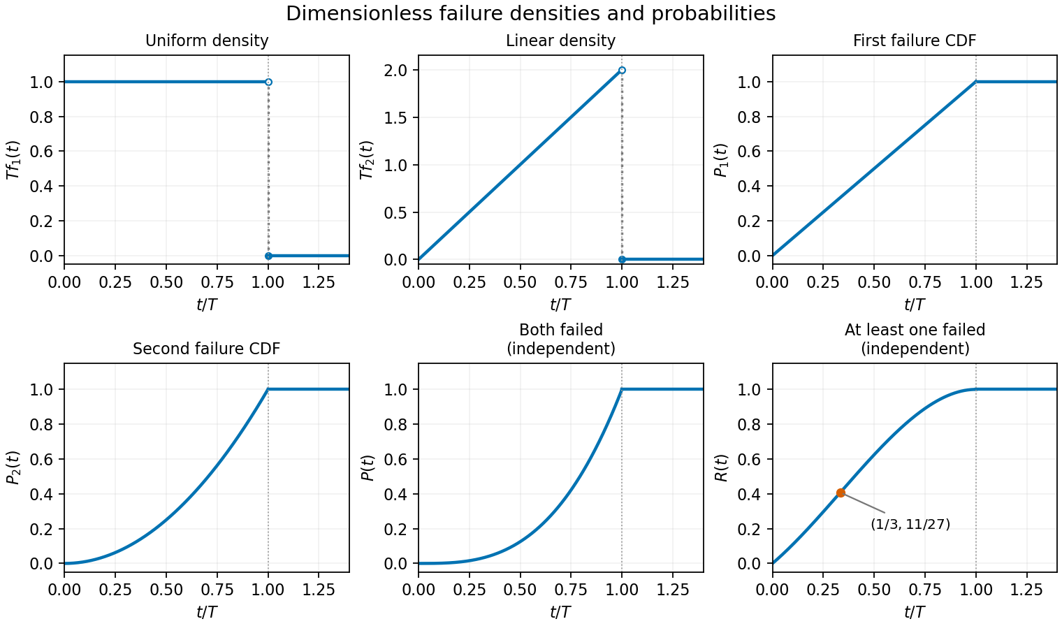
Without independence, $R=P_1+P_2-P$ still holds, but only $\boxed{s\le R(t)\le \min (1,s+s^2)}$ is forced by the marginals. Its inflection behaviour is then not determined. The shared-$U$ construction in (e), for example, gives $R=s$ before the plateau.

The product formula requires independent failure times. This assumption is not stated in the original PDF. Under that intended assumption, put $s=t/T$ and use the failure probabilities for two independent lifetimes:Its graph is a cubic increasing from $(0,0)$ to $(T,1)$, convex before reaching its plateau.

Without independence, the marginal distributions do not determine $P(t)$. The Fréchet inequalities give the sharp pointwise boundsFor example, taking $t_1=TU$ and $t_2=T\sqrt{U}$ with the same uniform random variable $U$ preserves both prescribed marginals but gives $P(t)=s^2$, rather than $s^3$.

The second cumulative distribution function is the integral of its density:Its graph is an upward-curving parabolic arc from $(0,0)$ to $(T_2,1)$, followed by a horizontal plateau. Both cumulative functions are continuous at their upper support endpoints.

Integrating the first probability density function gives the cumulative distribution functionIts graph is a straight ramp from $(0,0)$ to $(T_1,1)$, followed by a horizontal plateau.

Normalization requires $1={\int }_0^{T_2}Atdt=A{T}_2^2/2$. ThereforeThe graph rises linearly from zero to the left-hand limit $2/T_2$, then drops to zero beyond $T_2$. Its enclosed triangular area is one. The combined sketch in (f) uses dimensionless time and shows this density together with the cumulative probabilities.

A uniform distribution has constant density on its support, fixed by normalization. ThusThe density's assigned values at the endpoints do not affect probabilities.

Parametrize the diagonal by $\mathbf{x}(t)=(t,t,t)$ for $0\le t\le 1$. ThenThe second expression is $(t^3\cosh t{)}^{\prime }$, immediately giving $\int \mathbf{G}\cdot d\mathbf{x}=\cosh 1$. The first differs from it by $t^2\cosh t$. Two applications of integration by parts giveHenceThe changed value for $\mathbf{F}$ explicitly demonstrates path dependence, while $\mathbf{G}$ gives the same endpoint-dependent result.

On the first straight segment, $y=z=0$ and only $dx$ is nonzero, so both integrals vanish. On the second segment, $x=1,z=0$ and only $dy$ is nonzero; each integrand is one, contributing $1$. On the last segment, $x=y=1$ and only $dz$ is nonzero; each integrand is $\sinh z$, contributing $\cosh 1-1$. ThusThe second result also follows from the fundamental theorem for line integrals, using the potential found in (a). Agreement on this one path does not make $\mathbf{F}$ conservative.

The curl of the first vector field iswhich is not identically zero. Thus $\mathbf{F}$ is not conservative on ${\mathbb{R}}^3$ and cannot equal a negative gradient there.

For the second field, direct differentiation showsTherefore $\mathbf{G}$ is conservative, and the requested negative-gradient potential isIts curl vanishes, consistently with the curl of a gradient identity.

Use the same axes as in (a) and choose the outward orientation. On the curved spherical lune, $\mathbf{n}={\mathbf{e}}_r$ and $dA=a^2\sin \theta d\theta d\phi$. Its vector area isThe $y$ and $z$ components cancel. The $x$ component is $a^2(\pi /2)2\sin (\beta /2)$, henceHere ${\mathbf{e}}_x$ points along the azimuthal bisector; another coordinate choice rotates this vector accordingly. Its magnitude is the signed projected area, not the scalar curved area $2\beta a^2$. Reversing the orientation reverses its sign.

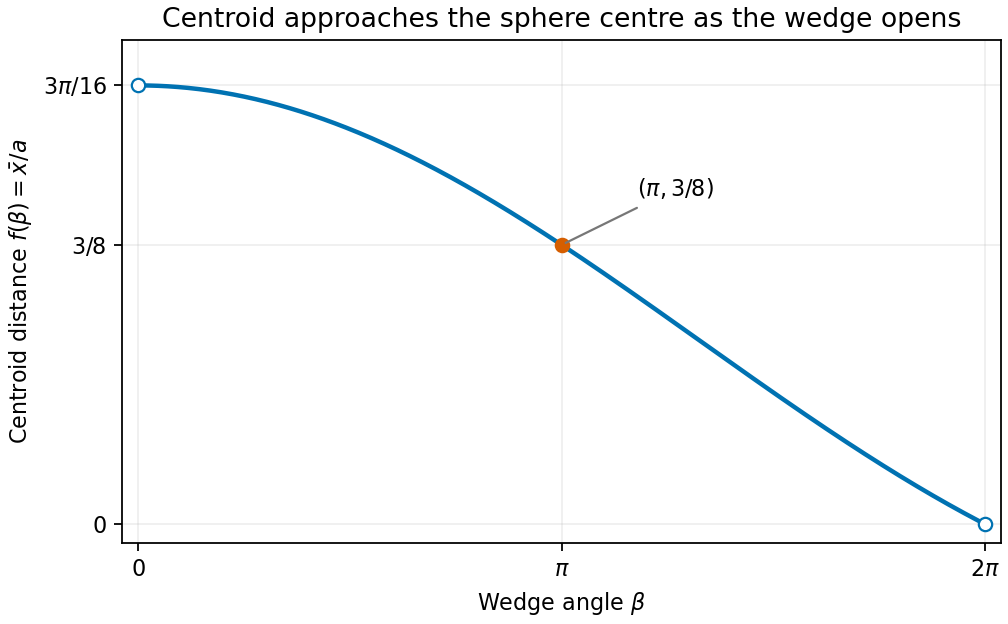
Orient the common axis of the wedge faces along $z$ and its azimuthal bisector along positive $x$. Reflection symmetries give $\bar{y}=\bar{z}=0$. In spherical coordinates, use $0\le r\le a$, $0\le \theta \le \pi$, and $-\beta /2\le \phi \le \beta /2$. The volume isSince $x=r\sin \theta \cos \phi$, the first moment isDividing by the volume locates the centre of mass:This is the centroid formula for a spherical wedge.

For the sketch, $f$ is positive and decreases from ${\lim }_{\beta \to 0^{+}}f=3\pi /16$ to ${\lim }_{\beta \to 2{\pi }^{-}}f=0$, with $f(\pi )=3/8$. Indeed, on putting $q=\beta /2$, the sign of $f^{\prime }$ is the sign of $q\cos q-\sin q$. The negative of this expression has derivative $q\sin q>0$ for $0<q<\pi$ and starts at zero, proving strict decrease.