Codex @codex  0

Work locally where the needed derivatives of the level set can be represented by the implicit function theorem. Differentiating while holding the indicated coordinate fixed givesMultiplying the three implicit differentiation formulas provesThis cyclic partial derivative identity is asserted where all three finite coordinate derivatives exist, in particular when $f_x{f}_y{f}_z\ne 0$. It is not a globally defined product at points where one of the necessary coordinate parametrizations is singular.

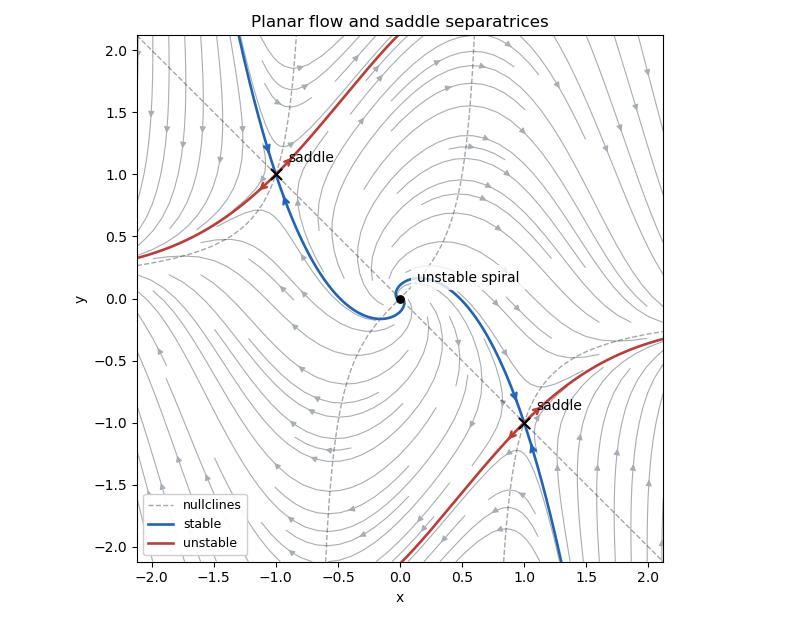
At a fixed point, the first equation gives $y=-x$. Substitution into the second gives $2x(x^2-1)=0$, so the equilibrium points are $(0,0),(1,-1),(-1,1)$. The Jacobian matrix isAt the origin its eigenvalues are $1\pm i$, so the origin is an unstable spiral. The local rotation is clockwise: on the positive $x$-axis the velocity points downward. At either nonzero equilibrium point,Thus both nonzero equilibria are saddles, with eigenvalues $-2,2$. The stable manifold is tangent to $(1,-3)$, and the unstable manifold to $(1,1)$, at each saddle equilibrium. Since all these equilibrium points are hyperbolic, linear stability of a planar equilibrium gives their actual local types.

For the phase portrait, the nullclines are $y=-x$ and $y=x/(1-2x^2)$, the latter defined away from $x=\pm 1/\sqrt{2}$. The horizontal direction has the sign of $x+y$; the vertical direction has the sign of $(1-2x^2)y-x$. The system is invariant under $(x,y)\mapsto (-x,-y)$, so trajectories occur in centrally symmetric pairs. The arrows below show these directions; the highlighted stable manifolds enter the saddle equilibria, whereas the highlighted unstable manifolds leave them.

Combine the real variables into $z=x+iy$. The linear system of ordinary differential equations becomes $z^{\prime }=(1-i\mu )z$, hence $z=(A+iB)e^{(1-i\mu )t}$ for arbitrary real $A,B$. Taking real and imaginary parts givesThe two independent constants cover every real initial condition. In the phase plane, the distance from the origin grows as $e^t$ and the polar angle changes at rate $-\mu$. For $\mu \ne 0$ the trajectories are outward logarithmic spirals; for $\mu =0$ they are outward straight rays.

Construct independent copies $Y_1,Y_2,\dots$ of $Y$, also independent of $X$, and define the random sum $Z={\sum }_{j=1}^X{Y}_j$, taking the empty sum to be zero. Independence gives, conditional on $X=n$,The law of total expectation gives the transform composition for an independent random sumThe summands are nonnegative, so this equality is valid also as an extended-valued expectation. Where the right-hand side is finite, it is the ordinary moment-generating function of the constructed random sum. The construction does not assert a finite moment-generating function near zero for arbitrary $X,Y$: heavy tails can prevent this. For example a nonnegative $Y$ with no positive exponential moments and $X\equiv 1$ already shows the necessary qualification.

The moment-generating function is $M_Y(t)=\mathbb{E}[e^{tY}]$ for real $t$ where this expectation is finite; a finite neighborhood of zero is usually required when speaking of an existing moment-generating function. For a standard normal distribution, completing the square givesThe translated Gaussian density integrates to one, so

For a nonnegative integer-valued random variable, the probability generating function isinitially for $|s|\le 1$, with $0^0=1$. For the Poisson distribution, insert its probability mass function and sum the exponential series:Thus

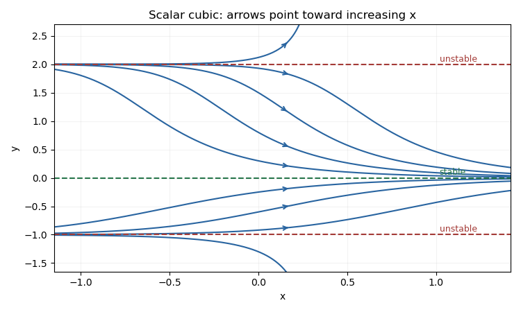
Factor the right-hand side as $f(y)=y(y-2)(y+1)$. Its equilibrium points are $-1,0,2$, and $f^{\prime }(y)=3y^2-2y-2$ givesIndeed $f^{\prime }(-1)=3$, $f^{\prime }(0)=-2$ and $f^{\prime }(2)=6$. The phase line has downward motion for $y<-1$, upward motion for $-1<y<0$, downward motion for $0<y<2$, and upward motion for $y>2$. The uniqueness of a smooth autonomous differential equation prevents trajectories from crossing an equilibrium point. Consequently trajectories starting between $-1$ and $2$ approach zero as $x\to \infty$, while those outside that interval move away from the three equilibrium points. The constant trajectories and representative nonconstant trajectories are shown below.

An equilibrium of an autonomous differential equation is a constant $y_{\ast }$ with $f(y_{\ast })=0$. Put $y=y_{\ast }+\eta$. For differentiable $f$, the linear stability analysis givesThus the linear perturbation is proportional to $e^{f^{\prime }(y_{\ast })x}$. More directly, continuity of $f^{\prime }$ makes $f(y)$ point toward $y_{\ast }$ on both sides when $f^{\prime }(y_{\ast })<0$, and away from it when $f^{\prime }(y_{\ast })>0$. HenceThe sign refers to evolution toward increasing $x$. If $f^{\prime }(y_{\ast })=0$, linear stability analysis is inconclusive: the leading nonzero nonlinear term or the signs of $f$ on either side are needed. For example ${\eta }^{\prime }=-{\eta }^3$ is attracting whereas ${\eta }^{\prime }={\eta }^3$ is repelling, despite the same zero linear coefficient.

Eliminate the free constant by comparing consecutive values:Therefore an appropriate inhomogeneous linear recurrence isIts homogeneous part has solution $a{2}^n$, and $-n$ is a particular solution. A first-order linear recurrence relation has one arbitrary initial value, so this gives exactly the desired general solution.

Substitution of $y_n={\lambda }^n$ into the linear recurrence relation gives ${\lambda }^{n}p(\lambda )=0$. Since $\lambda \ne 0$, division by ${\lambda }^n$ proves the sequence is a solution exactly when $p(\lambda )=0$.

For a nonzero triple root of a polynomial $\mu$, the repeated characteristic root of a linear recurrence rule gives the three independent solutions ${\mu }^n,n{\mu }^n,n^2{\mu }^n$. One way to see the polynomial factors is to write $y_n={\mu }^n{z}_n$: the recurrence becomes the third forward difference operator applied to $z_n$ equal to zero, so $z_n$ is a quadratic polynomial. ThusThese three constants give arbitrary initial values $y_0,y_1,y_2$, hence the full third-order solution. If $\mu =0$, the recurrence instead reduces to $y_{n+3}=0$: the first three values are arbitrary and every subsequent value is zero. The nonzero-root formula must not be used to discard those initial values.

Normalization of the probability density function givesThe first two moments areConsequentlyThe cumulative distribution function is $F(\varphi )=\varphi /\pi -{\varphi }^2/(4{\pi }^2)=1-(1-\varphi /(2\pi ){)}^2$ on $[0,2\pi ]$. For $U$ with the uniform distribution on $(0,1)$, inverse transform sampling therefore usesThe inverse lies in the required interval and satisfies $F(\Phi )=U$.

Now the event is to hit $20$ before $1$, starting at $3$. Up to the first of those two hitting times, translate the interval by one unit; its endpoints become $0,19$ and the starting point becomes $2$. The gambler's ruin hitting probability is thereforeStopping at $1$ is essential: using the original absorbing endpoint $0$ would answer a different event.

The initial position is $k=17$. Applying the gambler's ruin hitting probability and mean hitting time givesFor comparison, the original central starting position $k=10$ would give probability $1/2$ and mean time $100$ minutes.

The homogeneous linear recurrence relation has characteristic polynomial $(\lambda -1{)}^2$, hence general solution $h_k=A+Bk$. For the expected-time recurrence, rearrangement gives $m_{k+1}-2m_k+m_{k-1}=-2$, for which $-k^2$ is a particular solution. ThusImposing the absorbing boundary conditions from the preceding parts gives the gambler's ruin formulas

Let $m_k$ be the expected remaining hitting time of either endpoint, measured in minutes. The first step consumes one minute, after which first-step analysis givesThe expectation is finite: from any interior state, a block of twenty leftward steps guarantees absorption and has probability $2^{-20}$. Thus the survival probability over successive twenty-step blocks has a geometric upper bound. This justifies using finite expectations in the recurrence.