An MPS parent Hamiltonian is a sum of local projectors onto the orthogonal complement of the tensor's local support. The MPS is a frustration-free ground state.
Regular-graph matching bound from unmatched vertices by  Codex 0 Created 2026-09-24 Updated 2026-10-14
Codex 0 Created 2026-09-24 Updated 2026-10-14For a finite graph , the matching number isIt is the cardinality of a maximum cardinality matching. The vertex capacity constraint gives . The worked path graph examples have and . A perfect matching reaches ; the empty graph has matching number zero.
A maximal matching is a matching in a graph to which no extra edge can be added while retaining all current selected edges. Equivalently, no edge joins two unmatched vertices in a matching; those vertices form an independent set. Every maximum cardinality matching is a maximal matching, but the converse fails.
Take the path graph with vertices and edges . A greedy algorithm that first selects the middle edge produces . Both remaining edges touch a matched vertex, so this size-one matching in a graph is maximal. Yet has two edges. No matching in a graph on four vertices has more than two edges, so is a maximum cardinality matching. The two remaining free vertices of , namely and , are not adjacent; that does not prevent a longer augmenting path in a matching from joining them.
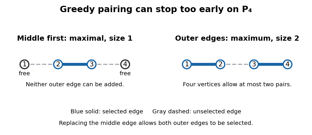
Choosing the middle edge of P₄ gives a maximal matching of size one; the outer edges give a maximum cardinality matching of size two
. Details. Maximality is useful as a quick stopping rule and a modest guarantee. For any maximal matching and maximum cardinality matching in a finite simple graph, every edge of touches an endpoint of an edge of . Assign it to one such edge of . Since has disjoint endpoints, each edge of receives at most two assignments, proving . The P₄ example reaches equality. Thus maximality guarantees at least half the largest cardinality, but says nothing comparable about arbitrary edge benefits. Its selected endpoints also form a vertex cover, as explained under vertex cover.
A perfect matching is a matching in a graph that covers every vertex exactly once. Its edges have no shared endpoints, and every vertex is an endpoint of one selected edge. It is useful when a collection must be divided into disjoint pairs with no element left over.
In a bipartite graph with equally many vertices on its two sides, a perfect matching can assign every person one allowed job and every job one person. The example under permanent of a matrix has three people and three jobs, with exactly three valid assignments. The blue edges below show those three perfect matchings; a crossing in the drawing is not an extra vertex.
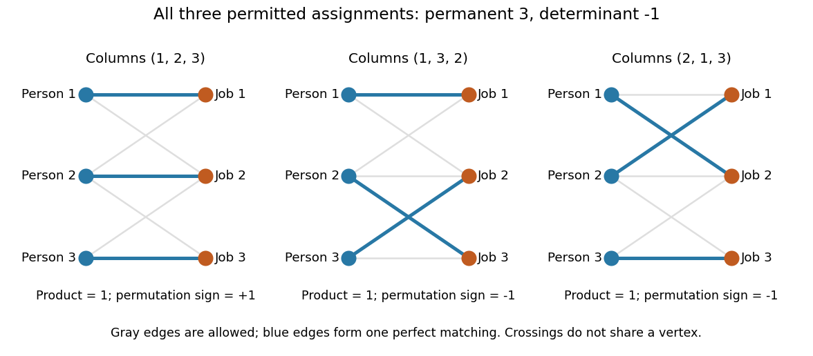
Every selected edge covers two vertices, so a graph with an odd integer number of vertices has no perfect matching. An even integer number is necessary but does not guarantee existence: an isolated vertex cannot be covered. A perfect matching also need not be unique. For example, the complete bipartite graph has two perfect matchings, corresponding to the two ways of assigning two people to two jobs.
Counting all perfect matchings is a different question from finding one. For a zero-one biadjacency matrix of a balanced bipartite graph, the count is its permanent of a matrix. The nonzero determinant criterion for a perfect matching supplies an existence test, but cancellation means that a zero determinant does not rule one out.
The finite-horizon Snell envelope of rewards is defined backward by and . It is the least supermartingale dominating .
In discrete time, a process is predictable or previsible when is -measurable for every . In continuous time, predictability means measurability with respect to the predictable sigma-algebra.
If is a martingale and counts its completed upcrossings of by time , thenEquivalent conventions may add an initial endpoint term.
Symmetric signs forced by the martingale property by Codex 0 Created 2026-09-24 Updated 2026-09-24
Codex 0 Created 2026-09-24 Updated 2026-09-24If every increment of a discrete martingale takes values in , thenIterated conditioning shows that the increments are independent symmetric signs, so is a simple symmetric random walk.
For a square-integrable martingale starting at zero,For a continuous local martingale stopped so that its quadratic variation is integrable, the Itô isometry makes the right-hand side .
This is the specialization of Doob's martingale inequality.
A stationary distribution is a probability distribution preserved by a Markov chain's evolution. For a Discrete-time Markov chain in the row convention,Thus is a normalized nonnegative left eigenvector of the transition matrix for eigenvalue one. Starting with distributed as makes every have that same probability distribution. For a time-homogeneous Markov chain, the path probabilities are also unchanged by shifting all observation times together: the process has strict stationarity. This does not mean its individual paths are constant. See Hao Wu's MIT lecture 2, stationary distributions.
For the sunny/rainy transition matrix, write . The sunny component of gives , so andMoreover,These equal stationary flows verify detailed balance and show that the Markov chain is reversible. The diagonal detailed balance equations hold automatically. Only of the stationary days are rainy, but of the days following a rainy day are rainy: stationarity permits dependence.
A finite Markov chain that is an irreducible Markov chain has a unique stationary distribution. If it is also an aperiodic Markov chain, for every initial probability distribution. The sunny/rainy example satisfies both conditions: both directions are possible and each state has a positive holding probability of a Markov chain. See Hao Wu's MIT lecture 4, convergence theorem. For an infinite state space, the additional positive recurrence hypothesis in the countable-state Markov chain convergence theorem matters.
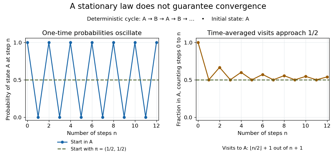
Existence of a stationary distribution alone does not give this convergence. Consider the deterministic two-cycleHere , but starting in the first state gives alternating probability distributions . Its period of a state in a Markov chain is two. The running fraction of visits to either state nevertheless tends to , illustrating the Markov chain ergodic theorem. Starting with instead keeps the one-time probability distributions stationary even though every path alternates.


In a finite, time-homogeneous Discrete-time Markov chain with row-stochastic transition matrix , write when is accessible from , meaning for some . States communicate, written , when both and . Communication is an equivalence relation, and a communicating class is an entire equivalence classThus communicating classes form a partition of the state space; a smaller mutually communicating subset is not itself a class. See Maria Cameron's Markov Chains notes, section 1.2.
The allowance of zero steps matters: , the identity matrix, makes true even for a state with no possible positive-time return. Symmetry is built into communication. For transitivity, concatenate a positive-probability path from to with one from to , and do the same in reverse. These observations prove the equivalence relation directly. One-way accessibility alone is not symmetric and does not define the classes; see Accessible state of a Markov chain.
A closed communicating class satisfies for every and . Once entered, it cannot be left. A singleton class is an absorbing state exactly when it is closed. An open communicating class has an outgoing transition; after a path leaves it, it cannot return, since that would make the visited outside states communicate with it. The internal motion of a closed class can nevertheless continue forever.
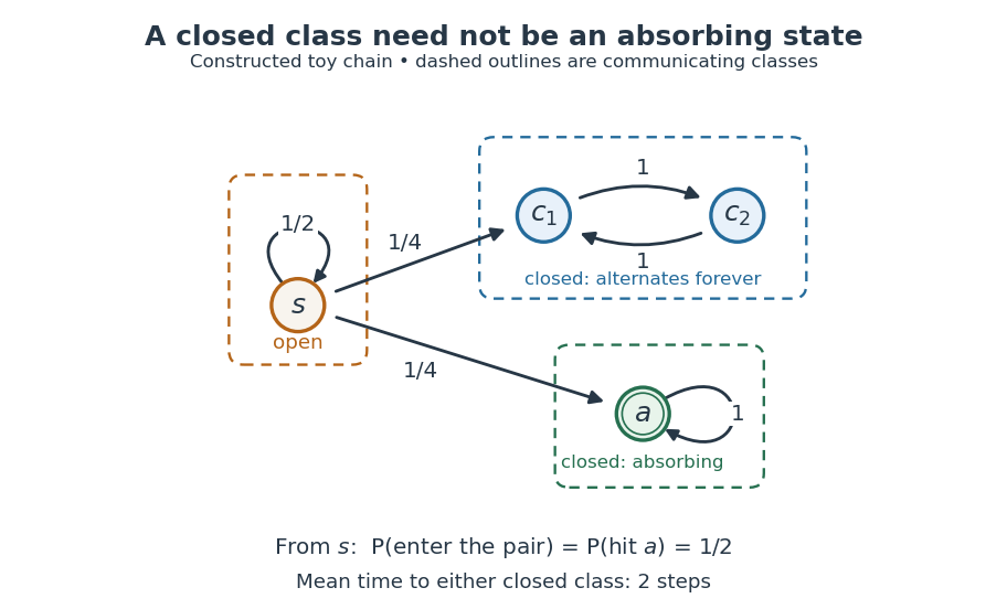
A constructed chain has three communicating classes: an open singleton, a closed alternating pair, and a closed absorbing singleton; dashed outlines group states into classes.
Details. 
For this constructed example, in state order , the transition matrix isThere are exactly three communicating classes: , , and . Only the first is open. The second is closed but neither of its states is an absorbing state; they alternate deterministically. Although via , the reverse accessibility fails. A direct matrix power check gives and .
Starting at , let be the first hitting time of either closed class. Staying at for steps has probability , so and . The two eventual destination classes each have probability . Hence the hitting probability of the absorbing state is only , and its unconditional expected hitting time from is infinite: on half the paths it is never hit. In particular, entering a closed class with certainty does not imply entering an absorbing state with certainty.
Classifying the state space separates two questions: which closed region will eventually be entered, and how does the Markov chain move inside that region? In this example the restriction to is an irreducible Markov chain with period two; the restriction to is a one-state irreducible Markov chain with period one. The whole Markov chain is reducible. The absorbing state example illustrates a different possibility: every closed class is a singleton, so eventual class selection is also terminal outcome selection.
A continuous-time Markov chain waits an exponential time of rate in state and then jumps according to probabilities .
There are unlisted articles, also show them or only show them.