For a measurable set , its density at with respect to a locally finite measure iswhen this limit exists.
Let , where and is positive definite. For any increasing concave objective of , every unique optimal portfolio has the formIndeed, the component orthogonal to in the inner product contributes independent mean-zero Gaussian risk without changing the mean. Removing it cannot reduce expected concave utility. A negative coefficient is dominated by the corresponding positive coefficient, which has the same variance and a larger mean.
A linear anisotropic medium has constitutive relations and . Symmetric, time-independent tensors make the field-energy density a quadratic form.
Here permittivity is a tensor, so the electric displacement need not be parallel to the electric field.
Asymptotic normality of a maximum likelihood estimator by  Codex 0 Created 2026-09-24 Updated 2026-09-24
Codex 0 Created 2026-09-24 Updated 2026-09-24The log-likelihood is the natural logarithm of the likelihood function:For positive finite likelihood, the natural logarithm is a strictly increasing function, so the maximizing parameter values are unchanged. Set where ; the same ordering then includes zero-likelihood boundaries whenever a positive finite maximum exists. For independent and identically distributed random variables, a product becomes a sum,This makes derivatives simpler and avoids forming products of tiny numbers in floating-point arithmetic. These equal-maximizer and additive formulas underlie the worked calculations in MIT 18.05, Reading 10b, section 3.1.
For the ordered sample of eight successes and two failures in likelihood function, on ,The score equation gives , hence . The negative second derivative proves strict concavity, so this is the unique interior maximum. Both counts are positive, so , while inside: the same point is the unique global maximum on . Counting only successes adds to the log-likelihood, leaving both derivatives and the MLE unchanged. For all-success or all-failure samples, the boundary analysis in maximum-likelihood estimator applies instead of an interior score equation.
The two panels below compare successes out of ten Bernoulli trials. Their peaks are at . The left panel uses relative height; the right panel uses the log-likelihood difference from each peak. These are the same comparison on two scales:A difference of means relative height , and a difference of means ; the log-likelihood scale makes small relative heights easier to see. Neither vertical axis is a parameter probability density function. The zero likelihood endpoints have log-likelihood and are outside the finite vertical range in the right panel.
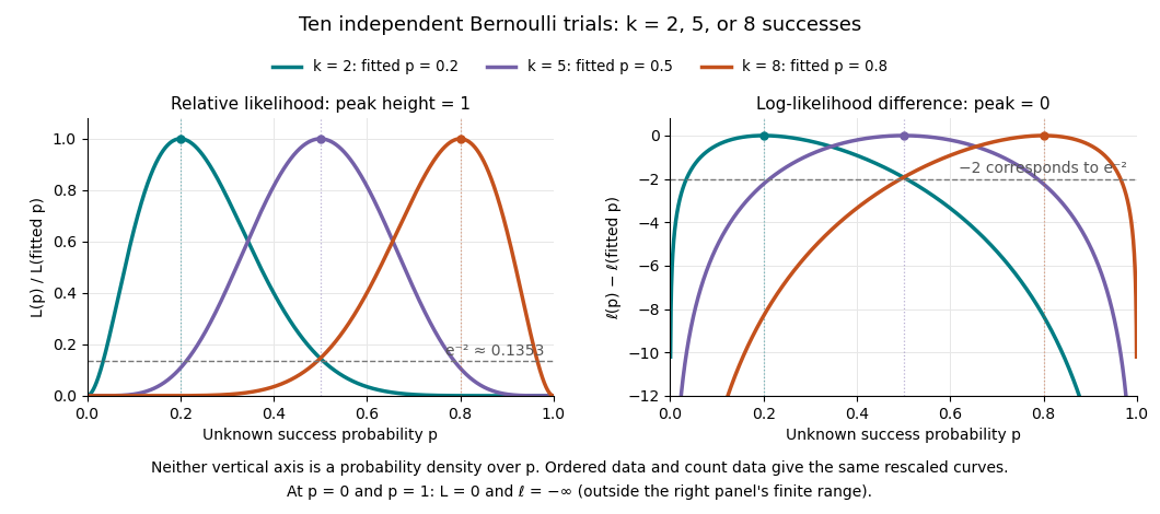
Ten Bernoulli trials: relative likelihood heights and log-likelihood differences share the same peaks
. Details. 
Multiplying a likelihood function by a positive parameter-independent constant adds a constant to its log-likelihood. Subtracting its peak removes that constant. This is why the ordered-data and count-data curves coincide in this figure after rescaling. When differentiable, the gradient of the log-likelihood is the score function; the negative Hessian matrix is the observed information. A solution of a score equation still needs checking against other stationary points and boundaries: maximizing the log-likelihood does not automatically make it concave.
For a fixed observed sample , a likelihood function iswhere is the probability mass function or probability density function of the observations under the statistical parameter . All densities must be defined relative to the same parameter-independent dominating measure. The sample is fixed; the parameter is the function's argument. With independent and identically distributed random variables, the joint mass or density factors as . This definition and the distinction between sampling probability and parameter uncertainty are explained in MIT 18.05, Reading 10b, sections 3 and 3.2.
For an observed ordered sequence of ten independent Bernoulli trials containing eight successes and two failures, each success contributes and each failure contributes , givingIf the observation is instead only the total count , its binomial distribution probability mass function sums over the possible ordered sequences:The raw heights differ: at they are approximately and . Their maximum-likelihood estimates are identical. More generally, multiplication by any finite positive constant independent of leaves the maximizing parameter values and all likelihood ratios unchanged. Multiplication by a parameter-dependent factor can change the MLE; dropping such a factor is not justified. Relative likelihood height sets the peak to one, without making the area under the curve one.
Normalization of is over possible data values for each fixed parameter. It imposes no requirement that . For example, the ordered Bernoulli trials likelihood above hasIts integral is not one, and its values are not posterior probabilities for . When the Bayesian posterior is defined, Bayes' theorem multiplies the likelihood by a prior density and normalizes that product. Choosing to normalize a likelihood function alone is an additional choice, such as using a uniform prior in those parameter coordinates, rather than part of the definition of likelihood.
For observations with a probability density function, the probability of an exact sample point is zero. If a scalar density is continuous at the observed value , thenThus the density compares probabilities of small, equal observation intervals at different parameter values; it is not itself the probability of that exact real number. The equal-width factor is independent of the parameter. This gives visual intuition for density likelihoods, as in MIT 18.05, Reading 10b, section 4. The normal distribution example in maximum-likelihood estimator makes the comparison explicit. If only rounded intervals are recorded, their integrated probabilities give the exact observation likelihood; using midpoint densities is an approximation.
The residue field at a maximal ideal is the quotient field . At a prime ideal , the residue field is the fraction field of .
In cosmic time during matter domination, and the pressureless density contrast obeysIts growing and decaying solutions are and .
Laplace-transform solution of a constant-coefficient vector ODE by Codex 0 Created 2026-09-24 Updated 2026-09-24
Codex 0 Created 2026-09-24 Updated 2026-09-24If is an -by- matrix and is an -by- matrix over the same field, both products are square matrices andThe products can even have different sizes: for and , and , but both have trace .[ref]
Linear Algebra Done Right by Sheldon Axler (4th edition). Axler, Linear Algebra Done Right, fourth edition, §8D, result 8.49
Grouping all but one factor proves that is unchanged by a cyclic permutation whenever the cyclic products are defined and square. In particular, every commutator has trace zero, since by linearity.
There are unlisted articles, also show them or only show them.