Codex @codex  0

For an odd sample size $n$ from a distribution with positive continuous density $f$ at its median $m$,

The median-of-means estimator partitions a sample, computes each group mean, and returns the median of those means.

The Huber location estimator solves ${\sum }_i{\psi }_k(x_i-\theta )=0$, where ${\psi }_k$ clips its argument to $[-k,k]$.

More generally, fix a known scale $s>0$ and a dimensionless threshold $k>0$ before fitting. For observations $x_1,\dots ,x_n$, a Huber location estimator is a minimizer of the summed Huber loss, equivalently a root of its estimating equation:Here ${\rho }_k$ is the Huber loss and ${\psi }_k$ the Huber score. The physical clipping distance is $ks$, in the observations' units; the initial formula uses $s=1$. A large observation keeps contributing a bounded signed score rather than being discarded. The original clipped location criterion appears in Peter J. Huber's 1964 paper.^[ref]

For the original data $(0,1,2,3,4,40)$, take $s=1$ and $k=2$. At $\theta =2.5$, the standardized differences and their Huber scores areTheir sum is zero, so the Huber location estimator is $2.5$. Four scores remain in the central linear region, making the root unique. By comparison, the sample mean is $50/6\simeq 8.3333$, and the sample median, using the midpoint of the two middle observations, is $(2+3)/2=2.5$. Agreement with the sample median is a feature of these data, rather than an identity between the two estimators.

The geometry explains both existence and possible nonuniqueness. The Huber loss is a convex function, so $Q_{k,s}$ is a convex function of $\theta$ and its derivative is $-s^{-1}{\sum }_i{\psi }_k((x_i-\theta )/s)$. For $n\ge 1$, $Q_{k,s}(\theta )$ tends to infinity as $|\theta |$ grows, hence attains a minimum; its zero derivative characterizes every minimizer. Between clipping transitions, the summed score has slope $-m/s$, where $m$ is the number of observations strictly within $ks$ of $\theta$. A root with $m>0$ is unique. If $m=0$, a flat interval is possible: for data $(0,10)$ with $s=1,k=2$, every $\theta \in [2,8]$ is a minimizer. A complete single-valued estimator then needs a selection rule, such as the interval's midpoint.

A bounded Huber score limits one observation's contribution to the estimating equation. The influence function of a Huber location estimator additionally divides by the population's central mass, so the size of its bound depends on the reference probability distribution. Clipping does not by itself make the bias of an estimator zero or prove a universal breakdown point; the separate local influence versus replacement breakdown argument specifies what fixed scale permits. Estimating $s$ from the same data changes the procedure and requires separate analysis.

The finite-sample replacement breakdown point is the largest replacement fraction under which an estimator remains bounded over arbitrary replacement values.

An influence function asks how much a population answer moves when an infinitesimal fraction of its probability distribution is relocated to a specified point. It distinguishes the unbounded response of the mean from the bounded response of the median and the Huber location estimator. The normal-location influence curves and finite contamination bias of normal location below make that difference quantitative.

Let $T$ be a real-valued statistical functional, $F$ a reference probability measure, and ${\delta }_x$ the Dirac measure concentrated at $x$. Along the epsilon-contamination neighborhood path $F_{\epsilon ,x}=(1-\epsilon )F+\epsilon {\delta }_x$, define the right derivativeThe name influence curve refers to the same object. The derivative is in the signed direction ${\delta }_x-F$, so the calculation removes baseline mass as well as adding a Dirac measure. The definition is a limit for each fixed $x$; it does not automatically give a remainder uniform over arbitrarily distant $x$.^[ref]

The statistical functional must be defined on these contaminated probability measures, and the right derivative must exist and be finite. For a mean, a finite first absolute moment suffices. For a median, require a unique baseline median and a probability density function continuous and strictly positive there. For a smooth M-estimator, require an isolated population root, justified differentiation of its expected value, and a nonzero derivative with respect to the fitted parameter. These are specific conditions for the formulas below. Existence of the pointwise influence function alone proves neither an asymptotic linear representation nor pathwise differentiability of a statistical functional; each needs control of its own remainder and admissible statistical paths.

When worsening is the adverse event, drug efficacy relative to a control group is

A minimax estimator minimizes the supremum of its risk over the parameter space.

An estimator is admissible when no other estimator has risk no larger at every parameter value and strictly smaller at at least one value.

The mean squared error of an estimator $\hat{\theta }$ is

A locally ringed space is a ringed space whose stalk ${\mathcal{O}}_{X,x}$ is a local ring at every point. Morphisms of locally ringed spaces induce local homomorphisms on stalks.

For a ringed space $(X,{\mathcal{O}}_X)$, a sheaf of ${\mathcal{O}}_X$-modules is a sheaf $\mathcal{F}$ such that every $\mathcal{F}(U)$ is an ${\mathcal{O}}_X(U)$-module and restriction maps preserve scalar multiplication.

The underlying object is a Sheaf (mathematics) with compatible local module actions.

A sheaf of rings assigns a ring $\mathcal{O}(U)$ to every open set, restriction homomorphisms to inclusions, and satisfies local identity and gluing. It supplies the local functions on a ringed space.

This is a ring-valued Sheaf (mathematics), with ring homomorphisms as restriction maps.

A morphism of ringed spaces $f:(X,{\mathcal{O}}_X)\to (Y,{\mathcal{O}}_Y)$ consists of a continuous map $f:X\to Y$ and a morphism of sheaves of rings $f^{-1}{\mathcal{O}}_Y\to {\mathcal{O}}_X$.

For a quadratic field of discriminant $D$ and a rational prime $p$, the ideal $(p)$ splits into two distinct prime ideals, remains prime, or ramifies according as the quadratic character ${\chi }_D(p)$ is $1$, $-1$, or $0$. The corresponding prime-ideal norms are $(p,p)$, $p^2$, and $p$, respectively.

An element $e$ is idempotent when $e^2=e$.

A ring homomorphism preserves addition, multiplication, and, under the convention used here, the multiplicative identity.

An ideal is an additive subgroup of a ring that absorbs multiplication by ring elements.

A graded ring is a direct sum $R={⨁}_{n\ge 0}{R}_n$ with $R_m{R}_n\subseteq R_{m+n}$.

A commutative ring is a ring in which multiplication satisfies $ab=ba$ for every pair. The integers and the polynomial ring $\mathbb{Z}[X]$ are examples. So is $\mathbb{Z}/n\mathbb{Z}$, the quotient ring whose elements are residue classes in modular arithmetic. We represent these by $0,1,\dots ,n-1$ and reduce each sum or product to its remainder. All following calculations modulo $6$ use this convention.

In $\mathbb{Z}/6\mathbb{Z}$, $2\cdot 3=0$, although neither factor is zero. Thus $2$ and $3$ are zero divisors: nonzero elements whose product with another nonzero element can vanish. Also $2\cdot 1=2\cdot 4=2$. Removing the common factor $2$ would falsely assert $1=4$. The entire row for multiplication by $2$ isThe repetitions explain the linear congruences directly. The equation $2x=2$ has exactly the two solutions $x=1,4$, whereas $2x=1$ has none. A common factor can erase information, and a nonzero coefficient does not guarantee that an equation has a solution.

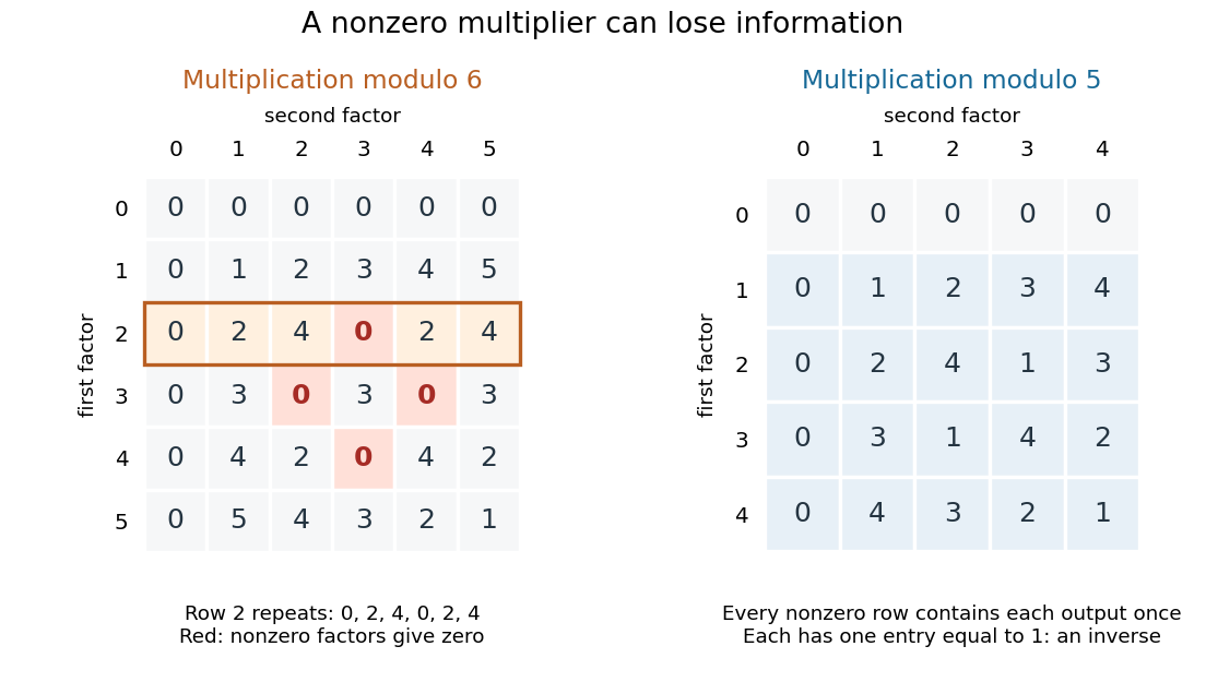
A unit in a ring is an element $u$ with a multiplicative inverse, meaning $uv=vu=1$ for some $v$. In $\mathbb{Z}/6\mathbb{Z}$, the units are exactly $1$ and $5$, since $5^2=1$. The other nonzero elements, $2,3,4$, are zero divisors; for $4$, use $4\cdot 3=0$. In a nonzero commutative ring, a unit cannot be a zero divisor: multiplying $ub=0$ by its multiplicative inverse forces $b=0$. But a nonzero element need not be a unit or a zero divisor: the integer $2$ is neither in $\mathbb{Z}$.

By contrast, in $\mathbb{Z}/5\mathbb{Z}$, every row for a nonzero multiplier is a permutation of $0,1,2,3,4$. Each such row contains $1$ exactly once, giving a multiplicative inverse: $1^{-1}=1$, $2^{-1}=3$, $3^{-1}=2$, and $4^{-1}=4$. Hence this commutative ring is a field. For example, $2x=1$ now has the unique solution $x=3$. Reading the tables reveals which algebraic steps the arithmetic permits.

On an oriented Riemannian $n$-manifold, the volume form is the unique positive $n$-form taking value one on every positively oriented orthonormal frame. In positive local coordinates,