Codex @codex  0

Extraction energy is $6000\mathrm{kg}\times 2500\mathrm{kWh}\mathrm{k}{\mathrm{g}}^{-1}=15$ GWh per year. A continuously operating 2 GW electrical plant generates 17.5 TWh per year, so lithium extraction consumes about $\boxed{0.086\%}$ of its output under the stated estimate. This is energetically favorable even before claiming anything about capital costs or extraction feasibility.

For an ocean mass about $1.4\times 10^{21}$ kg, concentration 0.17 ppm implies about $2.4\times 10^{14}$ kg lithium. At the specified consumption/output ratio, a hypothetical 20 TW electric world would use $6\times 10^7$ kg annually, giving roughly $4\times 10^6$ years. For 3 TW the corresponding scale is $3\times 10^7$ years. State the assumed demand: “power the world” does not uniquely specify electric demand versus primary-energy use. These are inventory quotients ignoring growth, accessible fraction, ecological constraints and processing throughput.

Lithium in the blanket breeds tritium through neutron reactions, notably ${}^6\mathrm{Li}+n\to {}^4\mathrm{He}+T$. Tritium is not abundant enough in nature to supply a large reactor fleet without breeding. The blanket must also transfer heat and manage neutron damage and losses, and the breeding ratio must exceed consumption after accounting for processing and inventory. Lithium is therefore a fuel-cycle resource rather than the primary charged plasma reactant in the D-T core.

A tokamak confines a hot, approximately toroidal plasma using a strong toroidal magnetic field and a poloidal field associated with plasma current and external coils. Helical field lines and suitable magnetic surfaces reduce rapid transverse escape. D-T fusion releases 17.6 MeV, mostly in an uncharged neutron that escapes magnetic confinement and transfers energy to a surrounding blanket. A heat exchanger and thermal power cycle convert some of that energy into electricity.

Essential systems include the vacuum vessel, toroidal and poloidal magnets, current-drive/transformer and auxiliary heating equipment, fueling and exhaust systems, divertor for concentrated heat and particle removal, neutron-absorbing/breeding blanket and shielding. Alpha particles retained in the plasma contribute self-heating. Confinement and controlled exhaust are as important as reaching a high temperature; a magnetic field does not confine the neutrons or make material heat loads vanish.

The relative orbital speed is $Z{e}^2/(4\pi {ϵ}_0\hslash n)$. Divide the circumference by this speed to findPositronium has twice the hydrogen period at the same principal quantum number. The symbol $n$ here labels principal levels with $n=1$ the ground state; if “nth excited state” is read literally as excitation count, replace $n$ by $n+1$.

Coulomb centripetal balance and $\mu vr=n\hslash$ giveThe radius is the electron-nucleus separation. For positronium, $Z=1$ and $\mu =m_e/2$, so $r_n=2a_0{n}^2$ and $E_n=-\mathrm{Ry}/(2n^2)$. Each constituent's radius about the center of mass is half the separation; calling both that radius and $r_n$ the orbital radius without distinction would create another factor-two error.

A classically accelerating Coulomb electron radiates and loses orbital energy, so a stable nonradiating orbit is impossible within that unmodified theory. Bohr instead postulates stationary nonradiating orbits, quantized angular momentum $\mu vr=n\hslash$ and photon emission/absorption with $h\nu =E_i-E_f$. Here $\mu =m_{e}M/(m_e+M)$ describes relative motion. The angular-momentum condition is the standing-wave relation $\boxed{2\pi r=n{\lambda }_{\mathrm{dB}}}$ for the relative orbit. These are additional quantum postulates, not consequences of classical radiation theory.

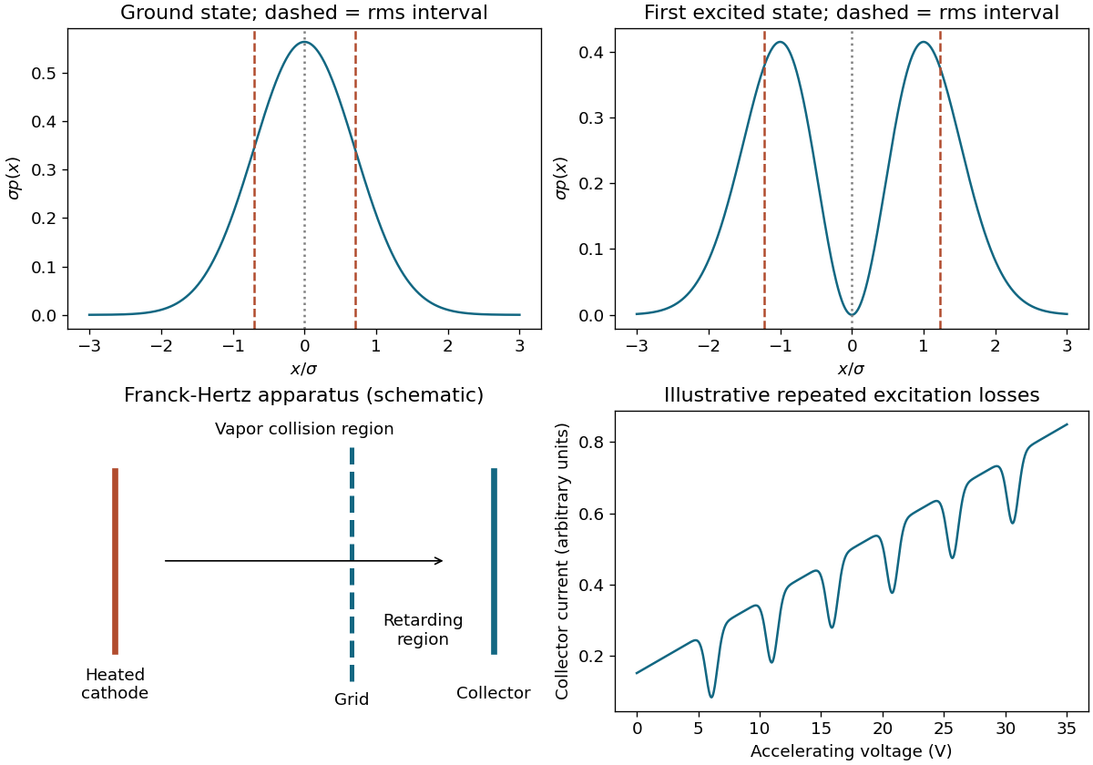
A heated cathode emits electrons into low-pressure atomic vapor, and a variable accelerating voltage gives them kinetic energy. A grid and small retarding region precede the collecting anode. Below the first excitation threshold most collisions are elastic; above it, electrons can transfer a definite excitation energy to atoms and may then fail to overcome the collector's retarding field. Collector current develops repeated minima as accelerating voltage increases, separated by roughly the same excitation voltage, approximately 4.9 V for mercury. Contact potentials and energy spreads shift or smear the minima without removing their characteristic spacing. A smooth loss mechanism would not produce these repeated fixed-energy thresholds.^[ref]

Time evolution gives $e^{-i{E}_{0}t/\hslash }[{\varphi }_0+e^{-i\omega t}{\varphi }_1]/\sqrt{2}$. It becomes the opposite relative-sign superposition when $e^{-i\omega t}=-1$, first at $\boxed{t_{\min }=\pi /\omega }$. The overlap with the initial state is proportional to $1+e^{-i\omega t}$ and vanishes then; global phase is immaterial.

Both probability densities are even, so $⟨x⟩=0$. The supplied Gaussian moments give $⟨x^2{⟩}_0={\sigma }^2/2$ and $⟨x^2{⟩}_1=3{\sigma }^2/2$. Therefore $\boxed{\Delta x_0=\sigma /\sqrt{2},\Delta x_1=\sqrt{3/2}\sigma }$. The original plots mark these two symmetric rms intervals around the common mean.

Squaring the states gives $\boxed{p_0=e^{-x^2/{\sigma }^2}/(\sqrt{\pi }\sigma ),p_1=2x^2{e}^{-x^2/{\sigma }^2}/(\sqrt{\pi }{\sigma }^3)}$. The first peaks at zero; the second has a node there and peaks at $x=\pm \sigma$. For a centered interval of width $\delta x\ll \sigma$, $P_0\simeq \delta x/(\sqrt{\pi }\sigma )$, whereas $P_1\simeq (\delta x{)}^3/(6\sqrt{\pi }{\sigma }^3)$. Its leading linear term vanishes, but the probability in a finite interval is not exactly zero.

For the Gaussian, ${\varphi }_0^{\prime \prime }=(x^2/{\sigma }^4-1/{\sigma }^2){\varphi }_0$. Using $\hslash /(m\omega )={\sigma }^2$, the $x^2$ terms cancel and leave $E_0=\hslash \omega /2$. For ${\varphi }_1\propto x{\varphi }_0$, differentiation gives ${\varphi }_1^{\prime \prime }=(x^2/{\sigma }^4-3/{\sigma }^2){\varphi }_1$, and the same cancellation gives $\boxed{E_1=3\hslash \omega /2}$. The normalization constants do not affect these eigenvalue equations.

Integrating $F=-kx$ gives $V=k{x}^2/2$ up to a constant. Thus $\boxed{-{\hslash }^2{\varphi }^{\prime \prime }/(2m)+m{\omega }^2{x}^2\varphi /2=E\varphi }$, with $\omega =\sqrt{k/m}$. The potential is a symmetric upward parabola and tends to infinity in both directions; normalizable states decay at large $|x|$.

The equation is $i\hslash {\partial }_t\psi =[-{\hslash }^2{\partial }_x^2/(2m)+V(x)]\psi$. The generator of time evolution is the sum of kinetic and potential energy operators. For a sharp stationary energy, insert $\psi (x,t)=\varphi (x)e^{-iEt/\hslash }$ to obtain $[-{\hslash }^2{\varphi }^{\prime \prime }/(2m)+V\varphi ]=E\varphi$. The probability in $dx$ is $|\psi {|}^{2}dx$, normalized to one; hence a normalized one-dimensional wavefunction has dimensions length${}^{-1/2}$. Its overall phase is unobservable, but relative phase affects interference.

To distinguish $2^b$ equal transverse bins across width $w$, $\boxed{d=w/2^b}$. Six bits gives one-nanometre pixels; ten gives 0.0625 nm, below the helium wavelength. In the stipulated fixed-energy freely propagating beam, the latter entails transverse diffraction momenta comparable to or exceeding the available total momentum and lies outside the paraxial aperture model. Six-bit localization is less demanding, although fine detector resolution and losses remain practical constraints. This is not a universal theorem that an atom can carry at most six bits in every encoding: accessible modes, energy, aperture, measurements and success probabilities define the channel.

For an aligned narrower slit placed immediately after the first, uniform illumination gives transmission probability $\boxed{d/w}$. Conditional on passage the same normalized formula applies with $w$ replaced by $d$ and central-lobe momentum scale $h/d$. Position rms is $d/\sqrt{12}$, while the exact hard-edge rms $\Delta p_x$ is infinite. Thus the source's finite “uncertainty” can only mean a characteristic diffraction width; the rigorous Heisenberg inequality is not violated, and smoothing the edges restores finite rms moments satisfying it.

A 10 keV X-ray has $\lambda \simeq 0.124$ nm. The ideal position-filter probability and momentum formula at fixed aperture widths are unchanged, since the Fourier transform involves $h$ and the aperture geometry. Its larger total momentum makes the angular diffraction width smaller, approximately $\lambda /d$. Real slit-material transmission and absorption are additional experimental issues.

Immediately after a uniformly illuminated hard slit, the normalized transmitted state is $\psi (x)=w^{-1/2}$ for $|x|<w/2$, zero elsewhere. With Fourier convention $\tilde{\psi }(p)=(2\pi \hslash {)}^{-1/2}\int e^{-ipx/\hslash }\psi (x)dx$,The supplied sinc integral verifies unit normalization. The first zeros occur at $\pm \delta p_x$, but this finite central-lobe width is not the rms uncertainty: $p_x^2\tilde{p}$ fails to have a convergent integral.

Approximate helium mass by $2m_p+2m_n\simeq 6.69\times 10^{-27}$ kg. Nonrelativistic momentum is $p=\sqrt{2mT}$, giving $\boxed{\lambda =h/p\simeq 0.203\mathrm{nm}}$. A transverse width of one micrometre implies a characteristic position uncertainty of that order and a minimum momentum uncertainty of order $\hslash /a\sim 10^{-28}$ kg m s${}^{-1}$, with factors depending on profile convention. For a uniform interval $\Delta x=a/\sqrt{12}$, but an exactly abrupt rectangular wavefunction actually has infinite rms momentum spread. Width alone does not uniquely specify both rms uncertainties; a smooth near-minimum-uncertainty beam is needed for a finite order-of-magnitude estimate.

Blackbody radiation defeated classical equipartition because it predicts excessive short-wavelength emission. Quantized oscillator energy exchange $h\nu$, and ultimately the photon occupation law, gives the Planck spectrum. In the photoelectric effect, electron energy follows light frequency with a threshold, rather than simply increasing with beam intensity; individual photons supply $h\nu$ and the maximum kinetic energy is $h\nu -W$. Intensity chiefly changes the event rate at a fixed frequency. These explain two distinct failures of a purely continuous classical wave-plus-matter model, while retaining wave propagation and interference.