The photoelectric effect is the release of Electrons from matter following photon absorption. Here the focus is emission from a metal surface into vacuum: a photon supplies energy, the work function pays the escape cost, and the remainder can become the emitted Electron's kinetic energy. A photocurrent counts collected electric charge; a stopping potential probes the upper kinetic energy limit. These are different measurements.
In 1905, Albert Einstein proposed that an individual light quantum could transfer its whole energy to one Electron. His §8 allowed losses before escape, distinguished the fastest emitted Electrons from the rest, and predicted a straight stopping potential versus frequency relation with a material-independent slope. He separately predicted that changing light intensity changes the number emitted without changing their velocity distribution under otherwise identical conditions. He also discussed incomplete transfer and limits to the account.[ref]
On a Heuristic Point of View Concerning the Production and Transformation of Light by Albert Einstein. Einstein's Miraculous Year; §8, printed pp. 193–196; full 21-page English translation of the 1905 paper
The useful modern starting model is a clean, homogeneous metal with independent single-photon events, negligible initial thermal broadening, negligible lowering of the surface barrier by an applied electric field, and negligible electric fields from the emitted Electrons themselves. Specify the surface and its work function; it is not enough to name the bulk material. The Einstein photoelectric equation describes the upper edge of the emission energy distribution. It neither predicts that every absorbed photon liberates an Electron nor supplies the whole photocurrent curve. Its appeal is that a complicated surface process still exposes the universal Planck constant through a simple slope.
For the ideal single-photon metal model, conservation of energy givesHere is the Planck constant, the incident frequency, the work function, and the largest emitted kinetic energy relative to the nearby vacuum level. An Electron at the highest occupied energy can reach this edge if it escapes without an additional loss. An Electron starting lower or losing energy within the metal emerges below it. The material takes recoil momentum; its recoil energy is neglected in this model.
For an original chosen example, take and . Using and the elementary charge gives and . The ideal stopping potential is therefore . At the same model supplies only per photon, so this single-photon channel is closed. A negative result from means no emission through that channel, not an emitted Electron with negative kinetic energy.
The photoelectric threshold frequency is the lower frequency boundary allowed by the ideal single-photon energy balance. With vacuum wavelength and speed of light , its corresponding longest wavelength is . The chosen work function gives and . These are model parameters, not a measured threshold for a named metal. Detectable photocurrent need not begin abruptly at the ideal boundary: collection, finite spectral width, thermal broadening and surface inhomogeneity matter.
A stopping potential is the magnitude of the retarding electric potential difference just sufficient to stop collection of even the fastest relevant Electrons in an ideal collection geometry. Since the Electron's electric charge is , the positive energy barrier is . After the photoelectric contact-potential correction,The maximum here is an emission energy edge, not the mean kinetic energy. In an ideal planar retarding geometry, transmission instead selects the component normal to the plates; identifying its endpoint with the full edge requires collection of trajectories that attain that edge in the relevant direction.
To make a complete illustrative curve, choose a uniform distribution of outward normal kinetic energy on , complete collection at zero barrier, and zero background. This is a deliberately chosen distribution, not a prediction of the Einstein photoelectric equation. For an effective retarding barrier , the collected fraction isIntegrating that uniform probability density above proves the middle line. Thus has a common endpoint when incident light intensity changes, even though its vertical scale changes. Real emission distributions need not give straight segments.
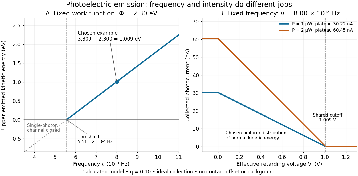
The photoelectric saturation current is the photocurrent reached when increasing the collecting electric potential difference no longer increases the fraction of available emitted Electrons collected. It is saturation with collecting voltage at fixed illumination. It does not mean that increasing incident light intensity cannot increase emission.
If is incident radiant flux on the emitting area and is the external quantum efficiency for producing escaping Electrons, then the incident photon arrival rate is and complete collection gives . For the example's , choose and . The calculated photon arrival rate is and . Doubling doubles this current to while leaving fixed. At fixed illuminated area this doubles the irradiance. Changing frequency at fixed changes the arrival rate as well as the photon energy; can also change, so there is no general rule that a higher frequency gives a larger photocurrent.
A missing plateau can indicate incomplete collection or an electric field altered by the emitted electric charge. Heating, surface changes and additional emission channels can invalidate a constant . Even a small amount of unwanted higher-frequency radiation can move an apparent endpoint. A stopping potential inferred from zero net current additionally needs background subtraction and a check for emission from the collector itself.
Robert Andrews Millikan's 1916 experiment used a magnetically turned wheel and rotary knife to expose sodium or lithium in vacuum. A surrounding copper-gauze/solid-copper collector caught Electrons; an electrometer recorded accumulated electric charge over thirty seconds at each applied voltage. He located endpoints graphically from photocurrent curves. Mercury spectral lines, selected by a monochromator and filters, controlled frequency; rejecting shorter-wavelength contamination protected the endpoint. An oxidized collector suppressed reverse emission for selected lines. A copper test plate measured the contact potential difference by a displacement-null method; a certified voltmeter set the electrical scale. He compared stable-surface sweeps with rapid alternating-frequency measurements to control drift. The slope tested ; the threshold required the contact correction. His gauge did not measure mercury vapor. Confirmation of the equation coexisted with his continued skepticism about localized light quanta.[ref]
A Direct Photoelectric Determination of Planck's h by Robert Andrews Millikan. §§2–3, pp. 361–367, Figs. 1–3; §4, pp. 372–375, Figs. 5–6; §5, p. 380; Theories of photo emission, pp. 383–385; publication verified by Caltech record 45t7b-bvc23: March 1916, Physical Review 7(3), 355–388
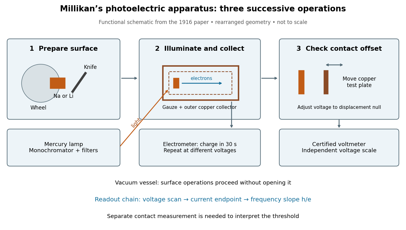
What Millikan photoelectric experiment controls and reads out
. Original functional reconstruction of the 1916 apparatus. Successive operations are separated and geometry rearranged; this is not a scale drawing. Source. Details.For a modern repetition of the logic, first establish electrical zero with the illumination blocked, characterize leakage, and verify the voltmeter scale independently of the presumed Planck constant. Scan several voltages near each endpoint rather than calling one noisy zero a cutoff. Hold the illuminated area and surface state fixed when varying light intensity; vary frequency independently when testing the slope. Repeating a reference frequency between other readings reveals time-dependent offsets. Agreement of a slope with tests an energy relation; it does not alone identify every microscopic step of photon absorption and escape.
A contact potential difference is an electrostatic electric potential difference associated with different conducting surfaces brought into electrical equilibrium. Surface condition and different work functions can create a vacuum gap field even when an external voltmeter reads zero. Connecting the metals establishes equilibrium of their electronic chemical potentials including electrostatic energy; it need not equalize the electrostatic electric potential in the gap.
Define as positive when the contact field adds to the retarding barrier, and let be the signed externally imposed retarding voltage. In this chosen sign convention the barrier is , henceThis convention specifies a model of the gap; an instrument's polarity labels must be translated into it. With a fixed , subtraction at two frequencies removes both the work function and the offset:For an original example with the same and an additional , choose and . The predicted terminal endpoints are and . The negative first endpoint calls for a small externally accelerating voltage because the contact field already over-retards the fastest Electrons. Their difference is , giving . Ignoring in the intercept would falsely infer for the work function. The terminal line's zero would then be mistaken for a material threshold. If drifts between the two readings, even the slope is biased. These are calculated examples, not Millikan's measurements.
The single-photon photoelectric threshold frequency is a regime-dependent statement. In multiphoton photoemission, multiple photons can supply the escape energy in one emission process. An ideal -photon energy balance would instead allow when , before additional losses or field effects. Thus increasing light intensity below the single-photon threshold cannot open that single-photon channel, but can make other channels relevant. The simple balance specifies neither their rates nor the illumination needed for them to dominate. Heating can also change the surface and emission mechanism. These cases require a different model from independent single-photon emission at a fixed work function.
Articles by others on the same topic

The photoelectric effect is a phenomenon in which electrons are emitted from a material (typically a metal) when it is exposed to electromagnetic radiation, such as light. The effect was first observed by Heinrich Hertz in 1887 and was later explained by Albert Einstein in 1905, which contributed to the development of quantum theory.



No matter how hight the wave intensity, if it the frequency is small, no photons are removed from the material.
This is different from classic waves where energy is proportional to intensity, and coherent with the existence of photons and the Planck-Einstein relation.