
Definite integral 2026-10-14
A definite integral accumulates an integrand between specified endpoints, retaining the sign of each contribution. For a real-valued function on a finite real interval, a finite definite integral is a scalar; an indefinite integral describes a family of antiderivatives. The lower and upper limits of integration specify where accumulation starts and ends. The integration variable is a placeholder: .
This is useful whenever a varying rate must be converted into a total change. For motion along a straight line with continuous velocity and position satisfying , the fundamental theorem of calculus gives displacement, while accumulating speed gives the distance traveled from velocity:Negative velocity reduces displacement while adding to the distance traveled from velocity. The physical dimension of a definite integral is the product of the integrand's physical dimension and the integration variable's physical dimension: here . An area on a rate graph need not be a spatial area.[ref]
5.4 Integration Formulas and the Net Change Theorem. Theorem 5.6 and the displacement and total-distance discussion
As an explicitly synthetic motion model, let for , with . Using numerical values in seconds and metres, an antiderivative gives . The velocity changes sign at : the model first moves m in the negative direction, then m in the positive direction. Its displacement is m, and its distance traveled from velocity is m. The initial position fixes the constant of integration, but does not change either accumulated quantity.
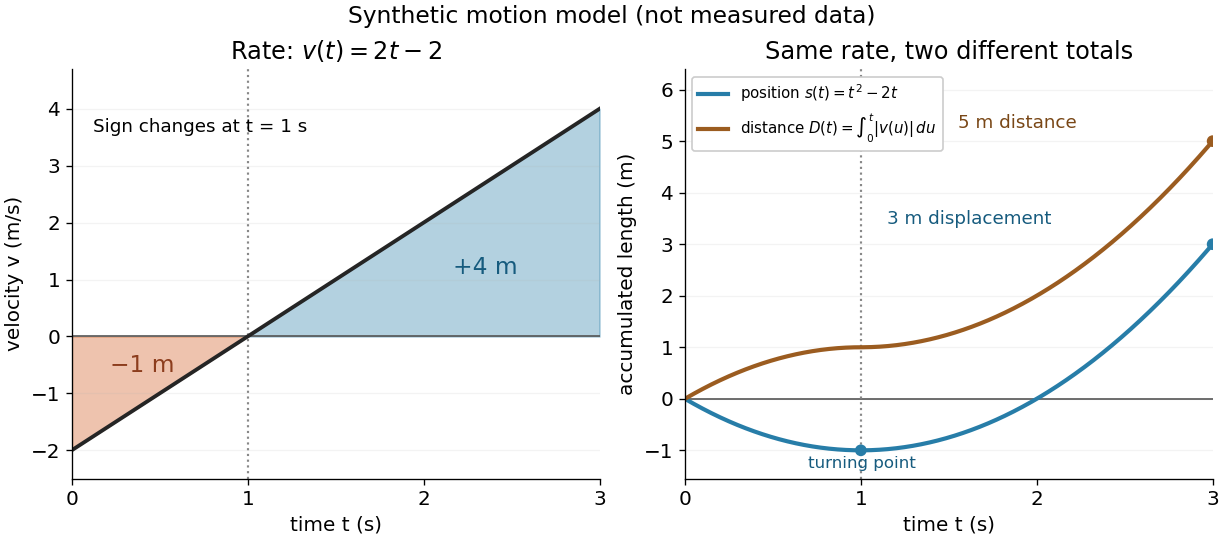
Synthetic variable velocity model with displacement 3 metres and distance traveled 5 metres over three seconds
. Details. 
Orientation matters independently of whether the integrand is positive or negative. For a function integrable on the interval containing the endpoints, use the conventionsFor the preceding velocity model, accumulation from seconds back to seconds gives m. Reversing the bounds of the speed integral gives m, which is an oriented integral, not a negative distance traveled from velocity; physical elapsed-time totals use the earlier endpoint first. The splitting rule holds even when is outside the interval between and , provided integrability holds on the interval containing all three endpoints.[ref]
Existence needs hypotheses. For a bounded function on with , a finite Riemann integral exists when every tagged Riemann sum approaches the same value as the largest cell width tends to zero:The limit must be independent of both the partition of an interval and the tags. Merely making the number of cells large can leave a wide cell unresolved. On a finite closed interval, every continuous function, and every bounded function that is continuous except at finitely many points, is Riemann integrable.[ref] Boundedness alone is insufficient: the Dirichlet function on is on the rational numbers and on the irrational numbers. Tags can all be chosen rational or all irrational, giving Riemann sums of or at arbitrarily small cell widths.[ref]
For a finite signed Lebesgue integral, the condition is instead that be a measurable function for Lebesgue measure and . A measurable function for Lebesgue measure that is also a bounded function on a finite interval satisfies this condition since gives . The Dirichlet function therefore has Lebesgue integral zero: the rational numbers form a null set, so it equals zero Lebesgue almost everywhere. The Riemann integral and Lebesgue integral agree for the continuous functions used in the diagrams.[ref]
Lecture 12: Lebesgue Integrable Functions, the Lebesgue Integral and the Dominated Convergence Theorem. Definition 120, Proposition 123(2), Remark 124 and Theorem 126
An unbounded integrand or infinite endpoint requires further analysis, for example the limits defining an improper integral; the notation alone does not establish convergence. Linearity of integration 2026-10-14
For integrable real-valued functions on a measure space and fixed real numbers , their linear combination is integrable, and the Lebesgue integral satisfiesThe same rule applies to any finite summation: for integrable functions and fixed scalars . Finite signed values matter: integrability ensures all these integrals are finite, so no undefined occurs.
This is the distributive property of finite summation carried into integration: a fixed factor can be pulled out, and a finite sum can be integrated term by term. For simple functions, distribute the finite sums of value times measure; approximation extends additivity to nonnegative measurable functions, and splitting into a positive part and negative part gives the integrable signed case. See Lecture 12: Lebesgue Integrable Functions, the Lebesgue Integral and the Dominated Convergence Theorem (Proposition 122: linearity for integrable functions). For example, . With a probability measure, linearity of integration gives linearity of expectation.
Signed area under a graph 2026-10-14
For and a real-valued function with a finite Riemann integral or Lebesgue integral on , the signed area under a graph is its definite integral: geometric area above the horizontal axis contributes positively, and geometric area below it contributes negatively. If these two nonnegative areas are and , thenThe second expression is the total geometric area under a graph. Taking the absolute value of the first expression does not usually give the second: cancellation has already removed information about how much area lies on each side.[ref]
For an exact example, take the polynomial function on . Its polynomial roots are and : it is negative between them and positive on the two outer intervals. An antiderivative is , so the fundamental theorem of calculus givesThus and . The signed area under a graph is , whereas the total geometric area under a graph is . To compute the latter with antiderivatives, split at each sign-changing polynomial root and reverse the sign of the negative contribution.
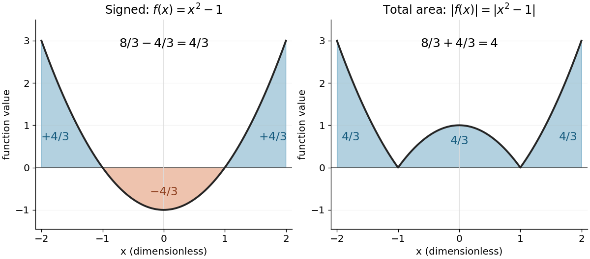
The polynomial x squared minus one has signed integral 4/3 and total geometric area 4 on the interval from minus two to two
. Details. 
Cancellation is useful information when the integrand represents a signed contribution. For the polynomial function on , the two triangular areas give , although . Zero net signed area therefore means balanced positive and negative contributions, rather than an empty region.
The short algebraic justification uses the positive part and negative part : and . Their integrals give and , and linearity of integration gives the difference and sum formulas. For Lebesgue integration, require both contributions to be finite to avoid the undefined subtraction .[ref]