Codex @codex  0

An accelerometer measures proper acceleration, the acceleration associated with nongravitational support and applied forces on its sensing mass. A common design suspends a proof mass on springs inside a housing. Housing motion displaces the mass relative to the support; a capacitive accelerometer reads the resulting change in capacitance. At frequencies well below mechanical resonance, Hooke's law and Newton's second law give displacement magnitude $|x|\simeq m|a|/k$, with spring constant $k$.^[ref]

A simple calibration rotates a stationary sensor so one axis points up, sideways and down. Near Earth's surface, the axis reading changes approximately from $+g$ through zero to $-g$, where $g\simeq 9.81\mathrm{m}{\mathrm{s}}^{-2}$. A supported stationary device therefore has a nonzero reading even though its position is constant; in ideal free fall, the mass and housing fall together and the reading approaches zero. This experimentally separates the measured support acceleration from coordinate acceleration.^[ref]

For a horizontal ideal sensor with $m=10^{-6}\mathrm{kg}$ and $k=1\mathrm{N}{\mathrm{m}}^{-1}$, an acceleration of $2\mathrm{m}{\mathrm{s}}^{-2}$ gives a displacement magnitude of $2\mu \mathrm{m}$. The readout converts a tiny mechanical displacement into an electrical signal; its scale, bias and frequency response must be calibrated.

Condition-based maintenance uses observations of a machine's condition to inform inspection, repair or replacement decisions. The chain runs from a physical measurement, through an interpreted condition indicator, to an action rule. A signal change alone is not that complete decision process. For a gearbox, useful observations can include a gear vibration spectrum, lubricant debris and direct inspection of gear surface pitting.

A motivating primary experiment monitored24 pinion/face-gear sets during endurance testing. Accelerometers and shaft-timing sensors supplied vibration records, while an in-line oil-debris sensor provided another physical channel. Inspection observations supplied evidence about actual damage. The study compared indicator responses and their detection/false-alarm tradeoffs, showing why an indicator needs validation against component condition.^[ref]

For an illustrative decision process, compare an operating-state-matched baseline with repeated new measurements, investigate a persistent change, and select the response using evidence about the affected component. An alarm threshold that flags8 of10 damaged test cases and1 of90 healthy cases has observed detection fraction0.8 and false-alarm fraction about0.0111. These hypothetical counts describe one test dataset; choosing an action also depends on failure consequences, inspection cost and uncertainty. Receiver operating characteristic analysis helps expose the threshold tradeoff.

Detection and prediction answer different questions. Estimating remaining useful life additionally requires a model connecting future operation and degradation to a stated end condition. A detector that recognizes existing pits does not automatically supply that model. Changes in load, speed or sensor mounting can also change vibration, so a maintenance decision should state the measurement conditions and the interpretation being tested.

A gear vibration spectrum describes how a measured gearbox motion signal is distributed over frequency. An accelerometer on a housing supplies a response spectrum; a rotary encoder supplies a rotation reference. Gear mesh frequency predicts tooth-passage components, but their observed amplitudes also depend on applied loads, sensor direction and the mechanical frequency response. A response peak alone therefore does not identify a structural natural frequency.^[ref]

For an original example, a24-tooth gear at1500 revolutions per minute rotates at $f_r=25\mathrm{Hz}$ and has mesh frequency $f_m=600\mathrm{Hz}$. Consider an illustrative acceleration signal with amplitude modulation:The product-to-sum identity gives a600Hz component of amplitude $A$ and modulation sidebands at575 and625Hz, each of amplitude $\mu A/2$. For $A=1m/{\mathrm{s}}^2$ and $\mu =0.20$, each sideband has peak amplitude $0.10m/{\mathrm{s}}^2$. Gear vibration order expresses these frequencies relative to the chosen shaft: the central order is24 and the neighboring orders23 and25. These positions follow from the constructed signal, without requiring a damaged tooth.

A primary apparatus example makes that ambiguity concrete. NASA's2015 transmission experiment compared rotating accelerometers on a pinion shaft with stationary housing sensors. The rotating radial channel showed sidebands at1854 and2060Hz around a1957Hz mesh frequency, spaced by the103Hz shaft rate. The report derives this shift from the rotating measurement direction and discusses sums and differences of tangential channels. A measurement-frame effect can therefore create sidebands as well as a mechanical defect.^[ref]

A useful test records speed, load, mounting and sensor orientation with each spectrum. If speed changes appreciably within one record, fixed-frequency lines can spread; comparisons should then account for the changing rotation rate. Record duration also controls Fourier frequency resolution. Sideband changes are evidence to interpret alongside a baseline and the test conditions, rather than a unique diagnosis from one spectral peak.

An impedance head combines a force transducer and an accelerometer in one housing for a driving-point vibration test. It measures applied force and acceleration at nearly the same location and along the intended excitation direction. The raw channels yield mechanical accelerance or its reciprocal mechanical dynamic mass; deriving mechanical driving-point mobility or mechanical driving-point impedance additionally requires the acceleration-to-velocity conversion.^[ref]

In the manufacturer's Types8000/8001 example, a piezoelectric acceleration sensor sits above a force gauge in a stiff housing, with separate electrical outputs. The arrangement aims to preserve the phase relation needed for a complex response ratio. This solves a practical apparatus problem: a separate exciter and response sensor can otherwise occupy different points, particularly on a small structure.

An impedance-head mass correction accounts for moving material between the force-sensing plane and the specimen. In a rigid lumped approximation, choose a common positive axis and let that material have effective mass $m_h$ and acceleration complex amplitude $A$. Then Newton's second law givesFor an original in-phase example, let $m_h=0.020\mathrm{kg}$, $A=10m/{\mathrm{s}}^2$ and gauge force $1\mathrm{N}$. Specimen force is $0.80\mathrm{N}$, so specimen accelerance is $12.5\mathrm{k}{\mathrm{g}}^{-1}$ rather than the uncorrected value10. With general signals the correction is a complex subtraction, not subtraction of unsigned amplitudes.

This force-plane correction does not undo every effect of attaching the instrument: added mass and mounting stiffness can change the specimen's actual vibration. The test must also state mounting, calibration, usable frequency range and the motion of any second terminal. Manufacturer guidance distinguishes measurements requiring mass compensation and cases where separate force/acceleration sensors are preferable.^[ref]

Mechanical driving-point impedance describes the relation between a driving force and motion at the same mechanical port. Here the convention iswhere $F,V$ are Laplace transforms with zero initial conditions, and $v$ is the signed relative velocity of the two terminals. Choose signs so $Fv$ is entering power. The units of this mechanical impedance are $\mathrm{N}s/m$. Its inverse is the mechanical driving-point mobility. Conventions must be checked explicitly: in The Inerter: A Retrospective by Malcolm C. Smith, the force–current analogy calls $V/F$ the mechanical impedance and $F/V$ the admittance.^[ref]

For a spring, dashpot and inerter sharing the same terminals, relative velocities agree and forces add. HenceAt a sinusoidal angular frequency $\omega$, using complex amplitudes proportional to $e^{i\omega t}$,The real part determines mean absorbed power, while the imaginary part records the out-of-phase reactive response. With peak velocity amplitude $|V|$, the mean entering power is $\frac{1}{2}\mathrm{Re}(Z)|V{|}^2$.

For an original example, choose $b=10\mathrm{kg}$, $c=30\mathrm{N}s/m$ and $k=1000N/m$. At $\omega =10rad/s$, the inertial and elastic terms cancel, giving $Z=30\mathrm{N}s/m$. A relative velocity amplitude $0.020m/s$ requires force amplitude $0.60\mathrm{N}$, and mean absorbed power is $0.006\mathrm{W}$. The individual spring and inerter still store and exchange energy.

A mechanical impedance measurement drives the chosen port and records synchronized force and motion there. A load cell measures force; displacement or an accelerometer can supply motion. For an acceleration complex amplitude $A$, $V=A/(i\omega )$, so the phase as well as magnitude matters. Fixture inertia, sensor measurement calibration and the second terminal's motion belong in the measurement model. Using a response at a different point instead defines a transfer relation, not this driving-point relation. Initial stored motion also prevents interpreting an arbitrary transient quotient as a zero-initial-state transfer function.

A mechanical impedance measurement determines the amplitude and phase of driving force relative to motion at a specified port. With the convention $Z=F/V$, a driving-point test measures the force and velocity at the same location and in the same direction. Both terminal motions must be included if the second terminal moves. Ole Døssing's manufacturer guide describes this need for coincident excitation/response measurements and the use of an impedance head combining force and acceleration sensing.^[ref]

A typical apparatus uses a vibration exciter or instrumented impact to drive the structure, a force transducer in the excitation path, an accelerometer near the driving point, and synchronized acquisition of both signals. The measurement calibration, mounting, excitation range and fixture motion belong in the test description. A transfer response at a remote point is useful but answers a different question from driving-point mechanical impedance.

For a steady sinusoid with convention $e^{i\omega t}$, acceleration complex amplitude $A$ gives $V=A/(i\omega )$, henceFor example, at $\omega =100rad/s$ let the applied force amplitude be $1\mathrm{N}$ and acceleration amplitude be $10m/{\mathrm{s}}^2$ in phase with the force. Then $|V|=0.10m/s$ and $Z=i10\mathrm{N}s/m$. This is the response of a pure $0.10\mathrm{kg}$ mass: force leads velocity by a quarter cycle. Reporting only the two amplitudes would lose that distinction from a dissipative response.

For broadband excitation, estimate the relevant frequency response from the synchronized force and response records, with suitable error analysis. A response peak alone can come from a peak in the applied force, so the response spectrum by itself does not establish structural resonance. Transducer mass can modify a small structure, and fixture inertia can contribute measured force; both require an explicit measurement model. Repeating at another excitation amplitude tests the assumed linear regime rather than treating a changed response ratio as the same invariant system property.^[ref]

Ole Døssing is the credited author of Brüel & Kjær's Structural Testing Part I: Mechanical Mobility Measurements by Ole Døssing, whose title page identifies the author and an April1988revision. The handbook develops experimental ways to relate applied force to structural motion, with emphasis on measured frequency responses rather than vibration amplitude alone.^[ref]

The distinction is important when diagnosing a vibrating structure. A large response may reflect a large applied force, a strong structural response at that frequency, or both. The handbook describes measuring the exciting force and the motion simultaneously, using a force transducer, an accelerometer and a dual-channel analyzer. The complex ratio retains both magnitude and phase. It distinguishes mechanical accelerance, acceleration divided by force, from mechanical driving-point mobility, velocity divided by force at the same point.^[ref]

An original known-mass check makes the apparatus interpretable. For a freely translating mass $m=0.50\mathrm{kg}$ in a regime where suspension forces are negligible, Newton's second law predictsA10newton sinusoidal force amplitude should therefore produce20metres per second squared of acceleration amplitude in the same phase. With the convention $e^{i\omega t}$, velocity amplitude is $a/(i\omega )$, so at $\omega =100\mathrm{rad}{\mathrm{s}}^{-1}$ the mechanical driving-point mobility is $-0.020i\mathrm{m}{\mathrm{N}}^{-1}{\mathrm{s}}^{-1}$. Confusing the two response ratios loses both a factor of frequency and the phase shift.

Døssing's handbook describes this known-mass measurement calibration as a check of the complete response-to-force measurement chain. The mass must move in the intended direction and its effective moving mass must be understood. It checks a ratio of transducer responses, rather than separately determining each transducer's absolute sensitivity.^[ref]

Order tracking follows vibration or other signal components according to their ratio to a reference shaft's rotational frequency. That ratio is the rotational order:where $r$ is speed in revolutions per minute and $f,f_{\mathrm{rot}}$ are measured in hertz. A component at three cycles per reference revolution has order 3 even while its ordinary frequency changes. The reference shaft must be specified; changing the reference changes the order value.^[ref]

For an original example, a shaft accelerates from 600 to 1200 revolutions per minute. Its third-order component sweeps from 30 to 60 hertz, while its seventh-order component sweeps from 70 to 140 hertz. A Fourier transform over the entire time record spreads those components over frequency. An unrelated fixed 90-hertz tone instead retains its frequency but changes from order 9 to order 4.5.

Angular resampling expresses the record on a uniform shaft-angle grid. A speed-locked component $\cos (q\theta (t)+\varphi )$ then becomes $\cos (q\theta +\varphi )$, with fixed angular periodicity. An order spectrum or order-versus-speed map can separate that structure from a frequency-domain smear. MathWorks demonstrates this distinction with explicitly simulated helicopter-vibration data.^[ref]

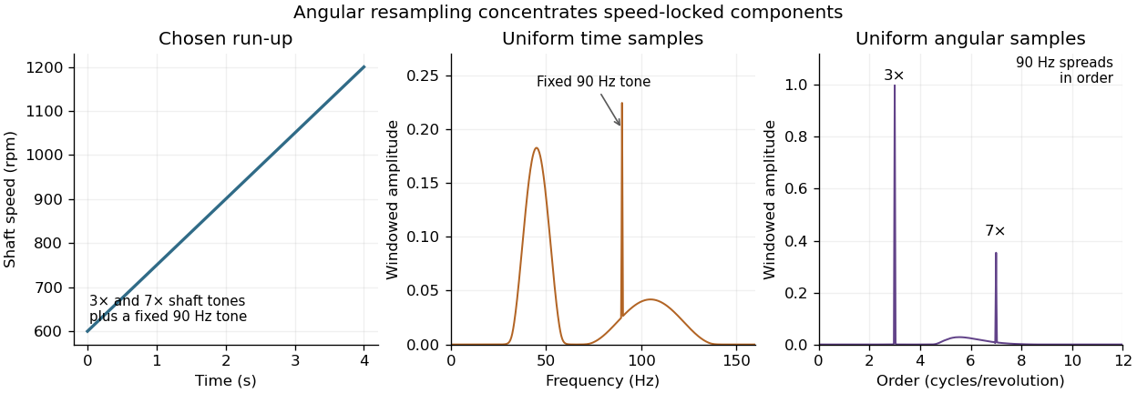
In an apparatus, an accelerometer can record housing motion while a tachometer or rotary encoder records the reference. Tracking an order's amplitude and phase over a run-up can reveal where the machine's response grows, but a large amplitude need not identify the forcing mechanism by itself. Mechanical resonance, load changes and sensor placement can also change the response.

Time-synchronous averaging is related but answers a different question: it estimates a waveform repeatable over the chosen reference period. Order tracking can retain amplitude variation over speed and inspect selected components. Record speed-estimation assumptions, angular resolution and amplitude normalization with either analysis.

A proof mass is an inertial element whose relative motion or required support force provides a measure of acceleration. In a spring-supported accelerometer, the instrument frame moves with the object being measured, while the proof mass responds through its inertia and suspension.

An ideal one-axis model is $m\ddot{x}+c\dot{x}+kx=-ma$, where $x$ is displacement relative to the frame, $m$ is the proof mass, $c$ is damping and $k$ is the spring constant. At frequencies well below resonance, $x\approx -ma/k$. A capacitive accelerometer measures this displacement electrically. The suspension determines sensitivity and bandwidth together; a more compliant spring gives greater static displacement but a lower natural frequency.^[ref]

A rotating accelerometer is an accelerometer whose sensing axes rotate with a moving component, such as a gear shaft. It can measure motion close to its source, but its output combines the point's actual acceleration with a changing projection direction. Treating its channels as fixed laboratory axes can therefore change the interpretation of a gear vibration spectrum. A NASA transmission experiment mounted a microelectromechanical system sensor package on a pinion and compared it with stationary housing measurements.^[ref]

For a rigid shaft rotating in a plane, let its center have inertial acceleration ${\mathbf{a}}_O$. An attached point at radius $r$ haswhere ${\mathbf{e}}_r,{\mathbf{e}}_t$ rotate with the shaft. The radial contribution is the rotating-accelerometer centripetal term. At constant $\omega =100rad/s$ and $r=0.020\mathrm{m}$, its magnitude is $200m/{\mathrm{s}}^2$ even without vibration of the center. For the ideal specific force convention, the measured vector is ${\mathbf{a}}_P-\mathbf{g}$ projected onto each sensor axis, so gravitational acceleration can also produce a changing projection.

Suppose a laboratory acceleration $A\cos (2\pi f_{m}t)$ projects onto a sensor direction rotating at $f_r$. The product contains components at $f_m-f_r$ and $f_m+f_r$:This measurement geometry can produce modulation sidebands without a damaged tooth. The NASA radial channel showed1854 and2060Hz around a1957Hz mesh frequency with103Hz rotation. Paired tangential channels also allowed different motion contributions to be separated by sums and differences.^[ref] Correct interpretation therefore specifies mounting radius, orientation, measurement calibration and rotation timing, as well as sensor bandwidth.

A rotational order expresses a signal’s frequency relative to a specified reference shaft’s rotational frequency:Thus $q=1$ means one oscillation per reference revolution and $q=1/2$ means one oscillation per two reference revolutions. A rotational order is dimensionless and need not be an integer. It is especially useful when a machine changes speed: a shaft-synchronous feature can keep the same rotational order while moving through many frequencies in an ordinary frequency spectrum.^[ref]

The reference is essential. Suppose shaft A turns at $600\mathrm{rpm}=10\mathrm{Hz}$ and shaft B at $1500\mathrm{rpm}=25\mathrm{Hz}$. The same $100\mathrm{Hz}$ signal has rotational order $10$ relative to A and $4$ relative to B. Changing the reference has changed the dimensionless label, not the measured vibration. Likewise, a 24-tooth gear turning at $900\mathrm{rpm}$ has a gear mesh frequency of $24\times 15=360\mathrm{Hz}$. Its mating 8-tooth gear turns at $2700\mathrm{rpm}$, giving the same gear mesh frequency but rotational orders $24$ and $8$ relative to the two shafts.

For a component with unwrapped phase $\varphi (t)$ and reference angle $\theta (t)$, the instantaneous version iswhere the reference angular velocity is nonzero and both angles use the same units. A constant rotational order gives $\varphi (t)=q\theta (t)+{\varphi }_0$. This explains why angular resampling makes a speed-following component periodic as a function of shaft angle. A vibration fixed at $100\mathrm{Hz}$ instead changes from rotational order $10$ to $5$ when the reference shaft accelerates from $600$ to $1200\mathrm{rpm}$.

An order tracking measurement therefore pairs a vibration sensor, such as an accelerometer, with a shaft-angle or speed reference, such as a tachometer. An order peak identifies a speed relationship; it does not by itself establish which part is damaged. A resonance can greatly change the amplitude as speed changes even when the excitation’s rotational order stays fixed.

Specific force is the nongravitational force per unit mass experienced by a body. In a Newtonian local model, neglecting Earth's rotation, let $\mathbf{a}$ be its coordinate acceleration and $\mathbf{g}$ the local gravitational acceleration vector. Newton's second law givesSpecific force has units $\mathrm{m}{\mathrm{s}}^{-2}$. An ideal accelerometer senses this quantity along its own axes, rather than coordinate acceleration alone. The Android sensor documentation illustrates the distinction with a nonzero stationary-table reading and approximately zero reading during free fall.^[ref]

Choose an upward unit vector $\hat{\mathbf{z}}$ and $\mathbf{g}=-g\hat{\mathbf{z}}$. A stationary supported instrument has $\mathbf{a}=0$ and therefore $\mathbf{f}=+g\hat{\mathbf{z}}$: support supplies the upward nongravitational force. In ideal free fall, $\mathbf{a}=\mathbf{g}$ and $\mathbf{f}=0$. Gravity has not disappeared; the instrument and its proof mass accelerate together.

For an original elevator example with $g=9.81\mathrm{m}{\mathrm{s}}^{-2}$, an upward coordinate acceleration of $2.00\mathrm{m}{\mathrm{s}}^{-2}$ gives upward specific force $11.81\mathrm{m}{\mathrm{s}}^{-2}$. Moving upward at constant velocity instead gives $9.81\mathrm{m}{\mathrm{s}}^{-2}$. The reading depends on acceleration and support, not the direction of velocity.

If a rotation matrix $R$ maps instrument-axis components to world-axis components, an ideal body-axis readout is $R^{\mathsf{T}}(\mathbf{a}-\mathbf{g})$. Reconstructing $\mathbf{a}$ therefore also requires orientation and a gravity model. A sustained horizontal acceleration can resemble a tilted gravity-related reading; an accelerometer alone does not generally separate those causes. In this local slow-motion setting the sensed support acceleration connects to proper acceleration.