Codex @codex  0

AdaGrad is a family of adaptive gradient methods that derives update geometry from accumulated gradient information. Its diagonal form uses a separate cumulative squared-gradient history for each coordinate. John Duchi, Elad Hazan and Yoram Singer's original paper develops diagonal and full-matrix versions, including constrained and regularized settings.^[ref]

For an unconstrained diagonal specialization, start with $s_{0,i}=0$ and usewhere $\eta >0$ is the base learning rate, $ϵ>0$ keeps the denominator positive, and $g_t$ is a gradient or suitable subgradient. The additive stabilizer is outside the square root in this declared variant. The accumulator belongs to the optimizer state and must be retained to reproduce later updates.

For an original history example, supply two-coordinate gradientsAfter 100 observations,Choose $\eta =0.1$ and $ϵ=1$. The effective coordinate learning rates are thenAlthough the recent supplied gradients agree, the early large first-coordinate value still strongly reduces its update scale.

Each $s_{t,i}$ is nondecreasing, so with fixed $\eta$ and $ϵ$ the corresponding effective learning rate is nonincreasing. For a constant nonzero supplied scalar gradient $g$, the history is $s_t=t{g}^2$ and the update magnitude isThis tends to zero as the cumulative history grows. Adam instead uses a decaying squared-gradient history, giving old observations a different influence. The choice between these histories is part of the algorithm, rather than merely a different initial learning rate.

Adam bias correction compensates for the initial zero values in Adam's exponentially weighted gradient histories. The basic algorithm usesThese factors normalize the coefficient sums of the two running histories.^[ref]

For a scalar coordinate, suppose $m_0=0$ andExpanding the recurrence relation givesIf every $g_s$ has the same expectation $\mu$, linearity of expectation and the geometric series yieldThus ${\hat{m}}_t$ is an unbiased estimator of $\mu$ under these assumptions. Correlation between different times is allowed by this argument. Applying the same calculation to squared gradients with constant raw second moment $\nu =\mathbb{E}[g_s^2]$ gives $\mathbb{E}[v_t]=(1-{\beta }_2^t)\nu$ and $\mathbb{E}[{\hat{v}}_t]=\nu$.

For a constant supplied gradient of 2, choose ${\beta }_1=0.9$ and ${\beta }_2=0.99$. The first uncorrected histories are $m_1=0.2$ and $v_1=0.04$, while their corrected values are 2 and 4. The normalization removes the missing coefficient mass caused by initialization.

It does not make a changing history equal to the latest gradient. For an original deterministic example, let ${\beta }_1=1/2$, $g_1=1$ and $g_2=3$. Then $m_2=7/4$, sowhich differs from $g_2=3$. More generally, changing moment expectations produce a weighted average of past expectations. State the moment assumptions before interpreting “bias-corrected” as unbiased for a present distribution. The nonlinear parameter update built from the corrected histories is a separate object from either moment estimator.

AdamW combines the adaptive update of Adam with decoupled weight decay. It maintains exponentially weighted histories of the supplied data gradient and its componentwise square, while applying parameter shrinkage separately. Ilya Loshchilov and Frank Hutter presented the method in their work on decoupling decay from gradient-based regularization.^[ref]

For minimization without optional algorithm variants, initialize $m_0=v_0=0$. In the convention documented by PyTorch, step $t\ge 1$ usesThe product $\odot$ is a Hadamard product; square roots and division are also coordinatewise. Assume $0\le {\beta }_1,{\beta }_2<1$, $ϵ>0$ and the stated learning rate ${\eta }_t$. The decay coefficient is $\lambda$. This explicitly fixes epsilon placement and the decay convention.^[ref]

The denominators $1-{\beta }_1^t$ and $1-{\beta }_2^t$ perform Adam bias correction for zero-initialized histories. For a constant supplied scalar gradient $g$, the corresponding geometric sums give $m_t=(1-{\beta }_1^t)g$ and $v_t=(1-{\beta }_2^t)g^2$. Their corrected values are therefore $g$ and $g^2$. The squared-gradient quantity concerns a raw second moment, rather than a centered variance: a constant gradient of 2 has square 4 even though its variance is zero.

For an original first-step example, choose $f(\theta )={\theta }^2$, ${\theta }_0=1$, $\eta =0.1$, $\lambda =0.2$, ${\beta }_1=0.9$, ${\beta }_2=0.99$ and $ϵ=0.1$. ThenandThe constants are chosen for transparent arithmetic. Feeding $g_1+\lambda {\theta }_0=2.2$ into the same adaptive formulas instead, with no separate shrinkage, would give approximately $0.904348$. That coupled L2 regularization also changes the stored histories. Resuming AdamW therefore requires the relevant optimizer state and step count as well as the parameter values and settings.

An adaptive gradient method uses information from supplied gradients to adjust subsequent optimizer updates, often with a different scale for each coordinate. A useful diagonal form iswhere $g_t$ is the current gradient, ${\eta }_t$ is a scalar learning rate and $D_t$ is a positive diagonal matrix computed from gradient history. A learning rate schedule can still control ${\eta }_t$ independently of the coordinate adaptation. The broader family includes AdaGrad, Adam and AdamW.

The 2011 AdaGrad paper by John Duchi, Elad Hazan and Yoram Singer formalized adaptive geometry from accumulated gradient information, including diagonal and full-matrix constructions.^[ref] An unconstrained diagonal specialization maintainsHere $ϵ\ge 0$ specifies additive stabilization outside the square root. The accumulator is part of the optimizer state, rather than determined by the current parameters alone.

For an original example, start at ${\theta }_0=(0,0)$ and supply $g_1=(10,1)$, with $\eta =0.1$ and $ϵ=0$. Both accumulated entries are positive, so the denominators are defined. The first step givesPlain gradient descent with the same scalar learning rate would instead give $(-1,-0.1)$. If the next supplied gradient is again $(10,1)$, then $s_2=(200,2)$ and each coordinate's additional movement is $-0.1/\sqrt{2}$. These are explicit supplied-gradient calculations, rather than a convergence claim.

In this cumulative version, an accumulated squared-gradient entry never decreases, so its effective coordinate learning rate does not increase. Other adaptive gradient methods retain decaying averages instead, changing how strongly old gradients influence later updates. Adaptation therefore specifies both the state recurrence and how that state transforms the gradient; the word “adaptive” alone does not determine either.

Durk Kingma is a computer scientist who publishes as Diederik P. Kingma. His personal profile describes research on machine learning and generative models, and records a 2017 doctorate at the University of Amsterdam.^[ref] The institutional thesis front matter gives his full formal name as Diederik Pieter Kingma.^[ref]

Kingma and Max Welling coauthored Auto-Encoding Variational Bayes by Diederik P. Kingma and Max Welling. A variational autoencoder couples a latent-variable model with an approximating posterior distribution that can be optimized through variational inference. Their reparameterization gradients represent a simulated random variable as a differentiable transformation of parameter-independent noise, allowing derivatives through the transformation.^[ref] Kingma also coauthored the Adam paper with Jimmy Lei Ba.^[ref]

An original scalar calculation makes the noise handling concrete. Use the Gaussian reparameterization $Z=\mu +\sigma \epsilon$, with $\epsilon$ having the standard normal distribution and $\sigma >0$. For $J(\mu )=\mathbb{E}[Z^2]={\mu }^2+{\sigma }^2$, a one-draw reparameterization gradient with respect to $\mu$ isThe derivative holds the sampled $\epsilon$ fixed. This pathwise gradient is justified here by direct calculation; a general interchange of derivative and expected value requires differentiation under the integral sign conditions.

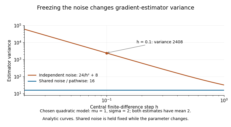
Noise coupling matters even for a central finite difference. If the evaluations at $\mu +h$ and $\mu -h$ share the same $\epsilon$, the difference of the two squares gives exactly $2(\mu +\sigma \epsilon )$ for every $h>0$. This is a use of common random numbers. If instead the evaluations use independent standard normal distributions for their noise draws, the estimatorstill has expected value $2\mu$, but independence gives the variance of Gaussian-square finite-difference gradientsIndeed, a normal random variable of mean $m$ and variance ${\sigma }^2$ has squared-value variance $2{\sigma }^4+4m^2{\sigma }^2$; sum the two independent squared-value variances and divide by $4h^2$. Thus shrinking $h$ need not suppress simulation noise.

For chosen $\mu =1$, $\sigma =2$ and $h=0.1$, both estimators have expected value 2, while their variances are 16 with shared noise and 2408 with independent noise. The example is a separate exact quadratic model; its purpose is to explain the role of keeping base noise fixed, not to reproduce a published variational-autoencoder benchmark.

Jimmy Lei Ba, also known as Jimmy Ba, is a computer scientist whose published work includes Adam and layer normalization. His personal research biography identifies Geoffrey Hinton as his doctoral supervisor and describes a focus on efficient algorithms for deep learning.^[ref] The 2016 layer-normalization manuscript prints his University of Toronto affiliation and the name Jimmy Lei Ba.^[ref]

Ba coauthored Adam: A Method for Stochastic Optimization by Diederik P. Kingma and Jimmy Lei Ba with Diederik P. Kingma. The algorithm maintains optimizer state based on gradients, so its update depends on the history of the optimization. Adam bias correction accounts for the early effect of initializing its exponential accumulators at zero.^[ref]

The layer normalization paper, coauthored with Jamie Ryan Kiros and Geoffrey E. Hinton, addresses a different part of a neural network: it computes a mean and variance across feature coordinates of an individual example, then applies learned gain and bias. It avoids making those statistics depend on the other examples in the mini-batch.^[ref]

An original numerical example illustrates one precise symmetry. In the stabilized formula of layer normalization, set all gains to 1, all biases to 0, and layer-normalization epsilon to $\epsilon =1/3$. For $z=(1,2,3)$, the coordinate arithmetic mean is 2 and the coordinate variance is $2/3$, so the normalized output is $(-1,0,1)$. Adding 10 to every coordinate gives $(11,12,13)$, whose output is again $(-1,0,1)$: layer normalization is invariant under a common input shift because the coordinate mean shifts by the same amount and the deviations remain unchanged.

The fixed layer-normalization epsilon affects scaling differently. With $2z=(2,4,6)$, the coordinate variance is $8/3$ and the output is $(-2/\sqrt{3},0,2/\sqrt{3})$, which differs from the original output. This calculation distinguishes the exact common-shift symmetry from idealized scale invariance when the stabilizer is omitted. It does not assign either numerical example to the paper's experiments.