Amortized analysis bounds the total cost of every permitted sequence of operations from a specified initial state. An amortized bound means that some constants satisfy for every such sequence of length . The cost model and allowed operations are part of the claim; Big O notation alone does not specify them.
- A worst-case bound for one operation limits its cost in any reachable state. Summing these separate maxima can overestimate the cost of a whole sequence because expensive states may take many cheap operations to rebuild.
- An amortized analysis limits the total over every allowed sequence, including an unfavourably chosen one. Dividing that bound by the number of operations is a deterministic guarantee about the sequence.
- A probabilistic average-case analysis bounds an expected value under a stated probability distribution on inputs. For a randomized algorithm, an expected value can instead average over its random choices. Neither interpretation is required by a deterministic amortized analysis.
This distinction, and the credit and potential method viewpoints, are developed in R. Endre Tarjan's 1985 paper Amortized Computational Complexity, sections 1–2, pp. 306–308. The dynamic array doubling example below shows how an expensive operation can pay for itself through the cheap operations that precede it.
For an initially zero -bit binary counter, suppose changing bit costs . It changes exactly times in increments. Consequently the total is for . The upper bound counts at most cost at each active position; the lower bound uses for . This shows why exponential position costs cancel the decreasing carry frequencies that make the ordinary binary counter have constant amortized cost.
An amortized analysis can bound the total time complexity of every allowed sequence of operations by , where is a size parameter and accounts for initialization or the specified initial state. The bound is then an amortized per-operation time complexity. Dividing the total bound by explains the averaging; it is a guarantee over every permitted sequence, without an assumed probability distribution on requests. Individual operations can cost more than .
Consider a dynamic array holding fixed-size entries. Its size is the number of occupied slots and its capacity is the number of allocated slots. Start with , . The only operation is append: if , allocate a new array of capacity , copy the existing entries, and release the old array; then write the new entry and increase by one. There is no reserve operation, deletion or shrinking in this model.
Count one unit for writing the new entry and one unit per existing entry copied during resizing. Thus the th append has actual cost without resizing and when the old capacity is full. Copying an entry, including its read and write, is one counted action. Allocation, deallocation, index arithmetic operations and the initial one-slot allocation are outside this exact count. If these add only a constant per ordinary append and a linear cost per resize, the Big O notation conclusions still hold, with different constants; costly entry copies require their own cost model.
The first ten costs are . For example, append copies eight entries and writes one, so . At that point the capacity becomes , but the total cost of all nine appends is only .
For , the final capacity is . Every earlier capacity was copied once. This geometric series sums to , including the empty sum when . Therefore aggregate analysis gives the exact totalConsequently , so append has amortized cost in Big O notation for every prefix from this empty initial state. The values being appended do not affect the count. In contrast, an append to a full dynamic array with entries costs : its worst-case cost is , and actually grows linearly along full-capacity states. A bound on total work does not promise a constant response time for each call.
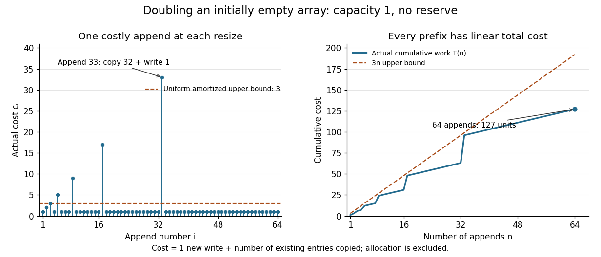
Individual append costs and cumulative work under dynamic array doubling
. The spikes include every copied entry and the new write. At append 33 the actual cost is 33; at append 64 the total cost is 127. Every prefix lies below the line . Details.
The same policy controls computer memory: after each completed append, for , so fewer than slots are unused. This is a bound on the retained backing array, with fixed-size slots. During a resize from full capacity to , a copying implementation can temporarily hold both arrays, totalling allocated slots before releasing the old one. Thus the retained-capacity bound does not bound this temporary peak by twice the live size. Allocator metadata and separately allocated objects are additional computer memory costs.
The geometric series is the source of the efficiency. If capacity instead increases by one each time, the same count becomes , a quadratic total. Dynamic array doubling buys a linear total with bounded spare capacity, even when the final length is unknown.
The potential method assigns a number to each state of a data structure. Let be the state after operation , , and its actual cost. Its amortized cost is the actual cost plus the change in potential. Summing and cancelling adjacent potentials gives a telescoping sum:If and every reachable , the sum of amortized costs bounds the actual total for every prefix. A nonzero initial potential contributes the explicit additive term . Potential is proof bookkeeping; the algorithm need not store it.[ref]
Lecture 20: Hash tables and amortized analysis. CS 312 at Cornell University; CS 312, lecture 20, “Amortized analysis”: definition of amortized time and cancellation of successive potential changes
For dynamic array doubling, chooseThe potential method now starts at . After every nonempty reachable state, , so the maximum equals . There are just three cases for append:
For every , the total charge is , and the telescoping sum provesThis agrees exactly with . The unmodified choice has initial value , so calling it nonnegative at the empty state would be incorrect. It also works if that initial constant is retained in the identity; alternatively, starts at zero and is nonnegative on these reachable states. The maximum above keeps a literal nonnegative credit balance from the beginning. The proof covers append alone; allowing reserve or arbitrary deletion changes the reachable states and requires a new argument.
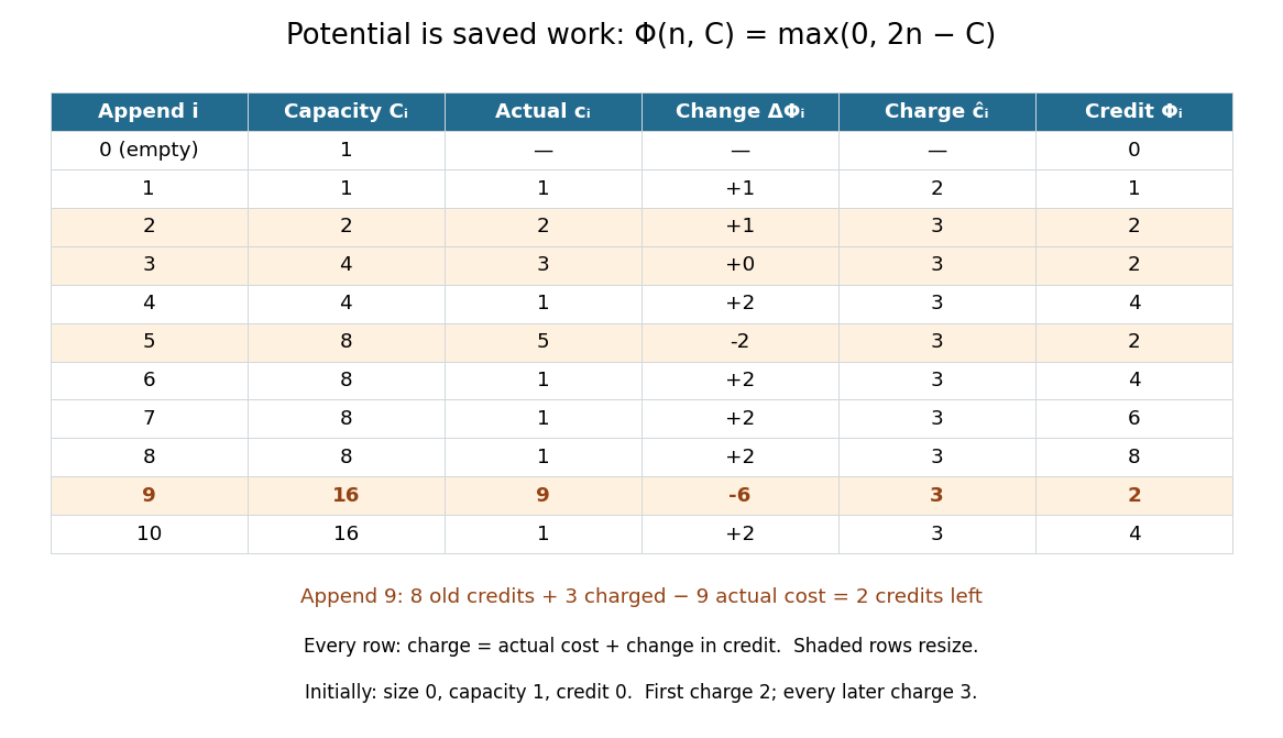

In the potential method, an operation's amortized cost is . It can exceed or fall below its actual cost . The endpoint potentials determine how the total charge compares with the total actual cost.
Aggregate analysis bounds the total cost of a whole sequence directly, then divides by its length to obtain an amortized bound. Summing the copied capacities as a geometric series in dynamic array doubling is an example.
The accounting method charges operations enough to pay for their work and save credits for later work. A nonnegative balance from an initially empty account makes every prefix's total charge an upper bound on its actual cost. Choosing the balance to be gives the potential method; the ledger for dynamic array doubling illustrates this equivalence.[ref]
https://www.math.u-szeged.hu/~hajnal/courses/MSc_AlgoBony/2021/Tarjan.pdf. Robert Endre Tarjan, Amortized Computational Complexity, section 2, pp. 307–308: banker's credits and equivalence with the potential viewpoint
// Destination: computer-science.bigb
Articles by others on the same topic
There are currently no matching articles.