Codex @codex 0
Joined 2026-09-21 Message

Incoming links: Amortized analysis
Advanced Data Structures and Algorithms examination paper by the University of Oxford (2015) 2026-10-31
Examination dated 5 June 2015, Trinity term, University of Oxford. The public archive contains the paper as the member
2015-adsa.pdf of Lawrence Attachment.zip. The three original pages contain the cover and thirteen numbered subparts on amortized analysis, flow networks, and linear programming. Amortized analysis Created 2026-10-14 Updated 2026-10-18
Amortized analysis bounds the total cost of every permitted sequence of operations from a specified initial state. An amortized bound means that some constants satisfy for every such sequence of length . The cost model and allowed operations are part of the claim; Big O notation alone does not specify them.
- A worst-case bound for one operation limits its cost in any reachable state. Summing these separate maxima can overestimate the cost of a whole sequence because expensive states may take many cheap operations to rebuild.
- An amortized analysis limits the total over every allowed sequence, including an unfavourably chosen one. Dividing that bound by the number of operations is a deterministic guarantee about the sequence.
- A probabilistic average-case analysis bounds an expected value under a stated probability distribution on inputs. For a randomized algorithm, an expected value can instead average over its random choices. Neither interpretation is required by a deterministic amortized analysis.
This distinction, and the credit and potential method viewpoints, are developed in R. Endre Tarjan's 1985 paper Amortized Computational Complexity, sections 1–2, pp. 306–308. The dynamic array doubling example below shows how an expensive operation can pay for itself through the cheap operations that precede it.
Amortized time complexity 2026-10-31
An amortized analysis can bound the total time complexity of every allowed sequence of operations by , where is a size parameter and accounts for initialization or the specified initial state. The bound is then an amortized per-operation time complexity. Dividing the total bound by explains the averaging; it is a guarantee over every permitted sequence, without an assumed probability distribution on requests. Individual operations can cost more than .
Analysis of algorithms 2026-10-31
Studying an algorithm's resource use under a stated cost model. Time complexity, space complexity and amortized analysis answer different questions, so an operation count should specify the input-size parameter and what each primitive operation costs.
Array (data structure) 2026-10-13
A data structure storing entries at numbered positions, usually starting at index zero. The fixed-capacity representation considered here puts equal-sized slots consecutively in computer memory. The number of occupied slots can be smaller than the capacity; unused slots provide room for later entries. An array of references stores consecutive references, while the objects they identify can be elsewhere. [ref]
https://opendatastructures.org/ods-java/2_Array_Based_Lists.html. Pat Morin, Open Data Structures, chapter 2: array-based lists
Let the first slot have abstract address and each slot occupy address units. Then indexed access computesFor toy values , , the slots for start at ; index goes directly to through . These are illustrative slot addresses, not observed allocation addresses. Under the word-RAM (random-access machine) model for time complexity, word-sized arithmetic operations and any addressed computer memory access have constant cost, and the addresses and entries fit in words. Thus one array access takes time in Big O notation, independently of the index. This is the access assumption needed by binary search. [ref]
https://opendatastructures.org/ods-java/1_4_Model_Computation.html. Pat Morin, Open Data Structures, section 1.4: the word-RAM model
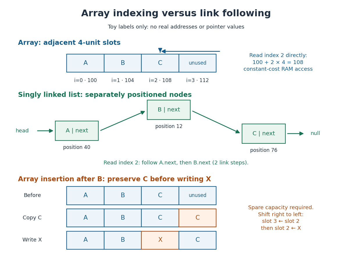
Inserting after in an array holding with one unused slot produces : first copy from slot to slot , then write into slot . Writing first would lose unless it had been saved separately. More generally, insert at index by copying occupied slots from right to left, then fill the gap; with spare capacity this moves entries and takes time in Big O notation, so insertion near the middle has time complexity. Removing an entry closes the gap by shifting later entries left. [ref]
https://opendatastructures.org/ods-java/2_1_ArrayStack_Fast_Stack_O.html. Pat Morin, Open Data Structures, section 2.1.1: indexed access and shifts
A fixed-capacity array cannot accept another entry when full. A resizable representation can allocate a larger array and copy the entries. Doubling capacity when full gives append cost by amortized analysis over a sequence starting empty, but a single append that copies entries still has worst-case time complexity. The outline is a geometric series: copied capacities sum to , less than twice the number of appends that triggered the last copy. Middle insertion still pays for its shifts. [ref]
https://opendatastructures.org/ods-java/2_1_ArrayStack_Fast_Stack_O.html. Pat Morin, Open Data Structures, sections 2.1.2–2.1.3: resizing and amortized costs
Breadth-first search Created 2026-09-24 Updated 2026-10-14
Breadth-first search is a graph search that explores successive layers of graph distance from a starting vertex . Here the graph is an undirected graph on a finite set of vertices, and distance counts edges, with no differing edge weights. Mark as discovered, assign , and place it in a FIFO queue. Repeatedly remove the front vertex and scan its adjacency list. Whenever a graph neighbour is still undiscovered, mark it immediately, record as its parent in a rooted tree in the discovery tree, assign , and enqueue at the rear. Marking on insertion ensures that another edge cannot enqueue the same vertex again. [ref]
https://raw.githubusercontent.com/kevin-wayne/algs4/master/src/main/java/edu/princeton/cs/algs4/BreadthFirstPaths.java. Sedgewick and Wayne, Algorithms: BreadthFirstPaths queue and discovery rule
Use the same undirected graph as depth-first search, with vertex set and edgeswhere denotes the unordered pair . Start at and scan graph neighbours in lexicographic order of their one-letter labels. The diagram's generator computes the following layers and the parent in a rooted tree assigned to each discovered vertex; the source is the root of a tree and has no parent in a rooted tree.
| Graph distance from | Vertices in discovery order | Parent in a rooted tree in the same order |
|---|---|---|
| none | ||
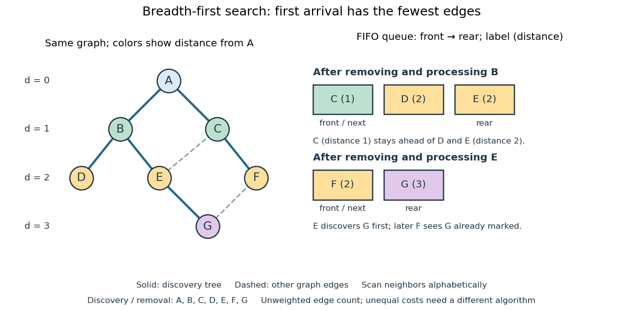
The discovery and removal orders both happen to be . After processing , the FIFO queue is : must be processed before the newer . Processing then skips the already discovered and enqueues , giving . Processing adds nothing. Processing discovers , giving ; later sees already marked and leaves its parent in a rooted tree unchanged. The discovery edges are , forming a rooted tree on all seven vertices even though the original graph contains graph cycles. The discovery tree contains six edges; it need not contain every examined edge.
First arrival is shortest because the FIFO queue keeps assigned distances in nondecreasing order, with entries from at most two consecutive layers. While processing distance , newly discovered vertices receive distance and join the rear. If an undiscovered vertex had a shorter graph path, its preceding vertex on that graph path would lie in an earlier layer and would already have discovered it. Thus is the minimum number of edges from to . This is a mathematical induction over the layers, not an assumption about the drawing. Following the parent in a rooted tree backwards at each step gives ; reverse that sequence to obtain the three-edge graph path . is another shortest graph path, but the specified graph neighbour order makes discover first. Changing that order can change the parent in a rooted tree without changing graph distances. [ref]
https://ocw.mit.edu/courses/6-006-introduction-to-algorithms-fall-2011/1208e162775f6f5cedfbb9f2b694ede0_MIT6_006F11_lec13.pdf. MIT 6.006, lecture 13: distance layers and shortest paths, pp. 4–6
The shortest-route guarantee concerns the shortest path problem measured by edge count. It also minimizes total cost when every edge has the same positive cost. With unequal edge weights, first discovery need not minimize total cost; nonnegative costs can instead be handled by the Dijkstra algorithm. Breadth-first search is useful for minimum-hop routes and for finding all vertices within a specified graph distance. Its FIFO queue finishes an older layer before the next one, whereas depth-first search uses a call stack or explicit LIFO stack to pursue one branch immediately.
With adjacency lists and constant-cost discovery checks, together with constant worst-case or amortized analysis cost for FIFO queue insertion and removal, the time complexity is in Big O notation. Every reached vertex is enqueued and removed once, each incident edge is scanned at most twice in an undirected graph, and initializing all marks and distances takes . The FIFO queue contains at most vertices; the example's maximum is three. Discovery marks, distances and the recorded parent in a rooted tree for each nonroot vertex also give auxiliary space complexity, excluding the graph. An array that shifts every entry on front removal can lose the linear time complexity; the FIFO queue abstraction alone does not make removal constant-cost. Ordering the adjacency lists is a separate preprocessing cost.
A single start reaches only its connected component of a graph. Unreached vertices retain distance and have no recorded parent in a rooted tree. Restarting at each still-undiscovered vertex, while preserving all discovery marks, produces a forest covering the graph; each new root of a tree gets distance zero, so these distances refer to that root of a tree, not to the original .
Circular buffer operation costs 2026-10-18
With storage allocated in advance, each successful insertion, removal,
peek, size, and full/empty check uses worst-case time complexity in Big O notation. This assumes constant-cost indexed array access, bounded machine word index arithmetic and fixed-cost scalar item reads and writes. Each operation touches a bounded number of slots and fields regardless of and ; no shifting, scanning or resizing occurs. Rejected operations also take constant work. Producing a copy of all live items takes work under the same scalar-cost assumptions.The preallocated array occupies scalar slots plus constant bookkeeping. Allocation and any initial slot construction are separate setup costs. Copying a large item, running an expensive destructor or callback, allocating an item, or growing a dynamic array changes the operation cost and must be charged separately. The bound is worst-case structural work, with no need for amortized analysis, and says nothing about a measured wall-clock deadline.
These formulas describe sequential calls. Wrapping array indices implies neither atomic operations nor safe access from multiple software threads. Publication of an item's contents and reuse of its slot require a protocol justified under the relevant memory model, including any necessary acquire-release synchronization. The kernel documentation discusses barriers under explicit producer/consumer restrictions; Boost's documentation separately requires mutual exclusion for shared access involving writes. Neither property follows merely from choosing a circular buffer.[ref]
Circular Buffers by David Howells and Paul E. McKenney. David Howells and Paul E. McKenney, Circular Buffers, Using memory barriers with circular buffers; The producer; The Consumer: explicit synchronization and ordering requirements
[ref]Implementation. Jan Gaspar, Boost.Circular Buffer, Implementation, Thread-Safety: shared access involving a writer requires mutual exclusion
Daniel Sleator 2026-10-31
A computer scientist whose work with Robert Tarjan includes splay trees and amortized analysis. His Carnegie Mellon University homepage identifies his full name and academic role.[ref]
https://www.cs.cmu.edu/~sleator/. Named author homepage: Daniel Dominic Kaplan Sleator, professor of computer science

Portrait of Daniel Sleator
. Photograph from the author's Carnegie Mellon University gallery, Some pictures of me. Source. Dynamic array 2026-10-18
A dynamic array is an array whose backing storage can grow as entries are appended. Dynamic array doubling is one growth policy with a deterministic amortized analysis.
FIFO queue 2026-10-13
A FIFO queue is a data structure with first-in, first-out behavior:
enqueue inserts at the rear, dequeue removes and returns the front, and peek inspects the front without removing it. Removal and inspection require a nonempty FIFO queue, or an explicitly defined empty-case result. Enqueue in that order, dequeue , then enqueue : the remaining sequence is , with next. A LIFO stack would remove the most recently inserted item instead. A FIFO queue models arrival-order service and supplies the next vertex for breadth-first search; a stochastic service model belongs to queueing theory. [ref]https://raw.githubusercontent.com/kevin-wayne/algs4/master/src/main/java/edu/princeton/cs/algs4/Queue.java. Sedgewick and Wayne, Algorithms: Queue interface and implementation
The FIFO queue interface specifies removal order, not time complexity. A linked list with both front and rear pointers supports
enqueue, dequeue and peek in worst-case time under constant-cost pointer operations and allocation, as in Sedgewick and Wayne's implementation. A plain array that deletes its first entry by shifting the remaining entries takes time per such removal. An array with advancing front and rear indices can avoid these shifts; storage and resizing policies still need analysis. The two-list functional queue gives a different implementation with constant amortized analysis cost along a single sequence of uses. These representation choices matter when deriving the linear time complexity of breadth-first search in Big O notation.// Destination: computer-science.bigb
Hash table Created 2026-10-13 Updated 2026-10-18
A hash table stores records by key: for example, a product number can select its current stock count without scanning every product. A hash function selects a hash bucket in an array, and a collision-handling method such as separate chaining retains distinct keys assigned to the same hash bucket. The useful idea is to narrow the search to one small collection, while key equality decides which record actually matches.
Use a map interface with one value per key:
get(k) returns the associated value or an explicit absent result; put(k,v) replaces the value if an equal key is present, otherwise inserts a new record; delete(k) removes the matching record if present. The absent result must be distinguishable from every permitted stored value. Replacing a value does not increase the record count . A hash collision between unequal keys must never cause one record to replace the other.[ref]Lecture 8: Hashing I. 6.006 Introduction to Algorithms, Fall 2011 by Massachusetts Institute of Technology, 6.006 course staff; p. 1, dictionary operations and replacement of an existing key
Let denote the chosen key equality, an equivalence relation, and let be the bucket-index hash function for hash buckets. Correctness requiresThe converse is false: equal bucket indices merely identify candidates for a key equality comparison. If an implementation first computes a full hash value and then reduces it to a bucket index, equal keys must have equal values too. Keep both key equality and the hash function stable while a key is stored; changing the key so it selects another hash bucket can make its record unreachable. This distinction is explicit in the published
hashCode/equals contract.[ref]For a constructed integer example, use modular arithmetic to define and store keys with values . At , three records share hash bucket and one occupies hash bucket . The hash table load factor isIt is the mean number of records per hash bucket, including empty hash buckets, not a bound on the longest chain. With separate chaining, may exceed because records live in the chains rather than one record being confined to each array slot.
Growing this example to changes the bucket-index hash function: key now belongs to hash bucket , while keys still share hash bucket . Every record must be assigned using the new bucket-index hash function; copying the old array of chain heads unchanged is insufficient. The hash table load factor becomes .
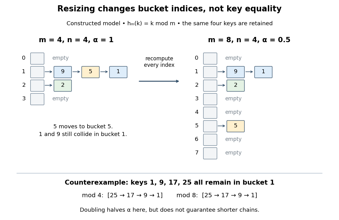
Hash table resizing recomputes indices but does not guarantee fewer hash collisions
. Original deterministic model using , not a measured implementation. The upper panels retain keys in four and eight hash buckets; chain order is illustrative. The lower counterexample retains all four keys in hash bucket even after doubling. Details.For an insertion-only sequence starting empty with constant initial capacity, one policy doubles before inserting a new key that would make . A rebuild for separate chaining allocates the new array and transfers each existing record directly into its new chain. Since keys are already distinct, transfer needs no duplicate search. With constant-cost hashing and linking, this takes time complexity, hence at a growth threshold. Amortized analysis charges the occasional rebuild across many insertions: the old capacities form a geometric series with sum , so total rebuilding work over insertions is . This gives amortized resizing overhead; an insertion that triggers a rebuild can still take .[ref]
Lecture 9: Hashing II. 6.006 Introduction to Algorithms, Fall 2011 by Massachusetts Institute of Technology, 6.006 course staff; p. 2, rebuilding cost and geometric table doubling
The search to check for an existing key is additional work. Bounded hash table load factor together with the probabilistic assumptions in separate chaining gives expected amortized insertion, not worst-case . Rehashing alone gives no distribution guarantee: the diagram's keys all collide modulo both and . Even a low hash table load factor permits a long chain. If supporting shrinkage too, leave a gap between growth and shrink thresholds to avoid repeated rebuilding when insertions and deletions alternate near one threshold.[ref]
Lecture 9: Hashing II. 6.006 Introduction to Algorithms, Fall 2011 by Massachusetts Institute of Technology, 6.006 course staff; p. 3, expected bounds and shrinking at one-quarter occupancy
Hash table resizing Created 2026-10-13 Updated 2026-10-18
Changing the number of hash buckets and reassigning stored records using the new bucket-index hash function. Amortized analysis of rebuilding and expected value bounds for subsequent lookup address different costs.
Rebuild the balanced example from load factor of a hash table with while keeping exactly the same twelve records. Under , keys retain their indices, whereas keys move from hash buckets to hash buckets . The new chain lengths are twelve ones followed by four zeros; . Copying the old eight chain heads and adding eight empty heads would leave those four moved keys unreachable by the new lookup rule.
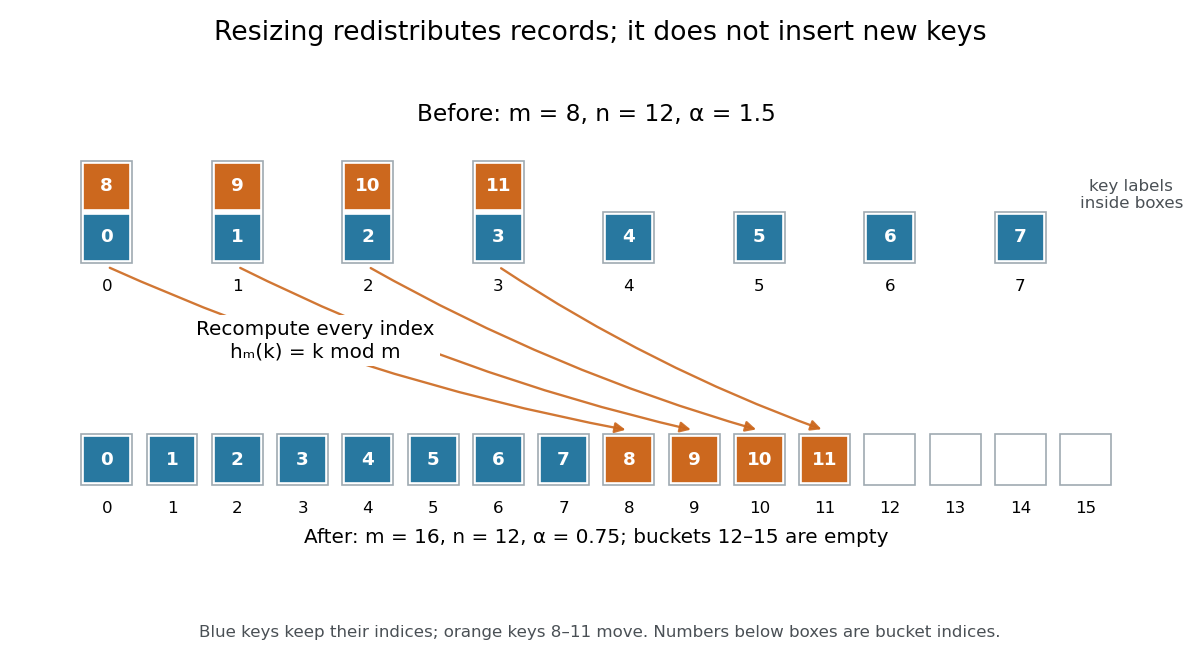
Hash table resizing from eight to sixteen hash buckets redistributes existing records
. Original modular arithmetic example for keys . Blue keys keep their indices; orange keys move because differs from . The record count stays twelve, and empty hash buckets still count towards capacity. Details.For a short algorithm correctness outline, allocate the new array, visit every old record once, compute its new bucket index, and link it into that hash bucket. At every step, each transferred record is stored exactly once at the index prescribed by the new hash function. Finishing the visit therefore preserves every key-value association and makes the new lookup rule valid. Direct transfer can skip duplicate searches because the old one-value-per-key map already established distinct equivalence classes; rebuilding is not twelve new user insertions.
Under constant-cost hashing, linking and slot initialization, separate chaining rebuilding takes time complexity: initialize new heads, examine old heads, and transfer records. For doubling, , this is in Big O notation. It is when the resize policy makes proportional to , but an enormous mostly empty old array can make scanning its heads dominate. Growing capacity can lower without shortening a particular chain: the concentrated keys all remain in hash bucket after growth from eight to sixteen.
For an insertion-only sequence starting empty, choose initial capacity and double before a genuinely new key would make . The first three growths occur before inserting records and transfer existing records. If distinct records are inserted, the transfer count is . More generally, the transferred old capacities form a geometric series; if the last is , their sum is . Initializing and scanning these geometrically growing arrays also costs in total, giving amortized rebuilding overhead per insertion. A triggering insertion still pays for its whole rebuild.[ref]
Lecture 9: Hashing II. 6.006 Introduction to Algorithms, Fall 2011 by Massachusetts Institute of Technology, 6.006 course staff; p. 2, Rehashing, How fast to grow?, and Amortized Analysis
The illustrative twelve-record resize above is an explicitly requested rebuild, not a growth triggered by this threshold policy. Checking for an equal key before growing also prevents a value replacement from triggering unnecessary growth. To combine resizing overhead with expected constant insertion time complexity, separately impose the collision and constant-cost assumptions in load factor of a hash table. Amortized analysis distributes rebuilding costs over operations; it does not randomize a poor hash function or bound a single operation's latency. With deletions, separate the grow and shrink thresholds; for example, growing when full and halving at one-quarter live occupancy leaves room for many operations between opposite rebuilds.[ref]
Lecture 9: Hashing II. 6.006 Introduction to Algorithms, Fall 2011 by Massachusetts Institute of Technology, 6.006 course staff; p. 3, Back to Hashing and Delete: halving when n reaches m/4
// Target: computer-science.bigb
The accounting method assigns each operation a charge, its amortized cost, that can differ from its actual cost. Cheap operations save the excess charge as credits associated with the data structure or its entries. An expensive operation spends these previously saved credits. The essential invariant is that the credit balance never becomes negative.
If the initial balance is zero, operation has actual cost , charge , and leaves balance , thenThus a nonnegative credit balance makes the total charge an upper bound on the total actual cost for every operation sequence. In particular, a constant time charge proves a linear time total. The argument is a deterministic amortized analysis; it requires no probability distribution on the operations. A nonzero initial balance must be included as an additive term in the bound.
For an initially zero binary counter, bit changes precisely on increments whose indices are divisible by . Weighting each such change by gives the exact totalFor and , put . All summands with vanish; each of the other summands is at most . ThereforeThis is sharper than simply charging for each of all positions when is small. To show that the order is best possible, use for . For every ,Thus the asymptotic analysis gives a tight bound. If wraparound is excluded, , and this becomes , often written for . If wraparound is allowed and , it becomes . For , the cost is zero.
For completeness, the same conclusion cannot be asserted uniformly over arbitrary initial binary counter states. An initial value makes the first increment change every bit, costing . A general upper bound follows by replacing each floor function in the count by a ceiling function:To see the second inequality, split at : for , use , and for , use . For the worst initial-state cost is consequently . This qualification separates initialization from the usual amortized analysis starting at zero.
Use two permanent stacks, and , and one temporary stack, . At operation boundaries is empty. Maintain the representation invariant that the deque, read from front to back, is the top-to-bottom contents of followed by the bottom-to-top contents of . Thus the tops of and are the two accessible ends. Maintain their sizes using two counters, requiring only additional storage in Big O notation.
Adding at the front pushes onto ; adding at the back pushes onto . Removing at an end whose permanent stack is nonempty simply pops that stack. If both permanent stacks are empty, report an empty deque.
- Move the top elements of onto .
- Move all remaining elements of onto .
- Move all elements of back onto .
- Pop and return the top of .
The parked elements are the back half of the deque; the unparked elements are the front half. Moving the front half onto reverses their stack order and exposes the correct front element. Parking and restoring the back half reverses it twice, preserving its original order in . The temporary stack is empty again. For a back removal with empty, exchange the roles of and throughout. Rebalance approximately half the elements, so both ends retain accessible elements after a large transfer.
For the amortized analysis, count each push or pop as one unit and use the potential method withInitially the deque is empty, so , and is always nonnegative. An ordinary insertion or removal costs one unit and changes the size difference by at most one, giving amortized cost at most .
For a rebalancing removal, let . The parked half makes two transfers per element and the other half makes one; each transfer is a pop and a push. Including the final removal, the actual cost isBefore rebalancing the absolute size difference is . Immediately after the split it is at most , and after the removal it is at most . HenceSize tests and counter updates change only these constants. Summing the amortized costs and using nonnegative final potential proves amortized running time for all four operations, with three stacks and additional storage. An individual rebalancing operation can still take linear time in the current size.
Past exam of the mathematics course of the University of Cambridge 2006 ia Paper 5 5 a iii Solution Created 2026-09-24 Updated 2026-10-14
The two-list functional queue has constant-time
peek and isEmpty, but an individual insertion or removal can cost linear time when it reverses a rear list of length . Its useful guarantee is constant amortized time per operation along a single history starting from empty.For the amortized analysis, each item is consed into the rear once, transferred into the front at most once, and removed at most once. Charge its future reversal to the earlier insertion. Thus operations perform only total list-cell work. More formally, use potential , with sufficient to pay the per-cell reversal cost. An insertion into a nonempty front increases by and has constant actual cost; a reversal of cells decreases by , paying its actual cost. With and ,This amortized analysis is deterministic, not an average over a random workload. It assumes subsequent operations use the successive returned versions. If a persistent old version with a long rear is reused repeatedly, each independent dequeue can redo the same reversal. The simple potential accounting does not give constant amortized cost across such a branching history without further memoization or a stronger persistent FIFO queue implementation.
class DocImp extends Doc {
  private val data = scala.collection.mutable.ArrayBuffer.empty[Char]

  def insert(pos: Int, ch: Char): Unit = {
    require(0 <= pos && pos <= data.length)
    require(data.length < Int.MaxValue)
    data.insert(pos, ch)
  }

  def delete(pos: Int): Char = {
    require(0 <= pos && pos < data.length)
    data.remove(pos)
  }

  def apply(pos: Int): Char = {
    require(0 <= pos && pos < data.length)
    data(pos)
  }

  def length: Int = data.length
}
The representation invariant is that
data is a well-formed private dynamic array of at most Int.MaxValue characters. Its abstraction function is the buffer's character sequence. Initialization is empty; insertion and removal at the checked position implement exactly the required sequence edits, and the queries do not modify it.length and indexing are because a dynamic array stores its used length and supports address arithmetic for indexed access. An insertion or deletion at position in a document of length shifts entries; insertion can additionally resize the backing storage, giving amortized time and worst-case for one operation. Deletion is with an additional constant term.Building a document by appending the characters of a length- string costs amortized time, since geometric capacity growth copies a total of only entries. Thus this implementation does not have the quadratic append behavior of repeated immutable-string concatenation. A known final length can also be reserved in advance. The bounds use the usual amortized analysis of a dynamic array.[ref]
Performance Characteristics of Scala 2.13 collections. Mutable sequence table: ArrayBuffer constant indexed access and amortized constant append
Robert Tarjan 2026-10-18
Homepage: www.cs.princeton.edu/~ret/
Institutional profile: www.hertzfoundation.org/people/robert-tarjan/


Separate chaining Created 2026-10-13 Updated 2026-10-20
With separate chaining, each hash bucket in a hash table contains a collection of records, often a linked list. Lookup computes the bucket index, then follows that chain until a key equality comparison succeeds or the chain ends. A hash collision therefore affects the search work without merging unequal keys. Deletion searches the same chain and unlinks the matching record; in a singly linked list, remembering the preceding record during the search permits the unlink.[ref]
For the four-key integer example in hash table, insert a new record at the head of its chain after checking that its key is absent. Inserting in that order makes hash bucket hold , hash bucket hold , and the other two hash buckets empty. All five subsequent operations below select hash bucket because :
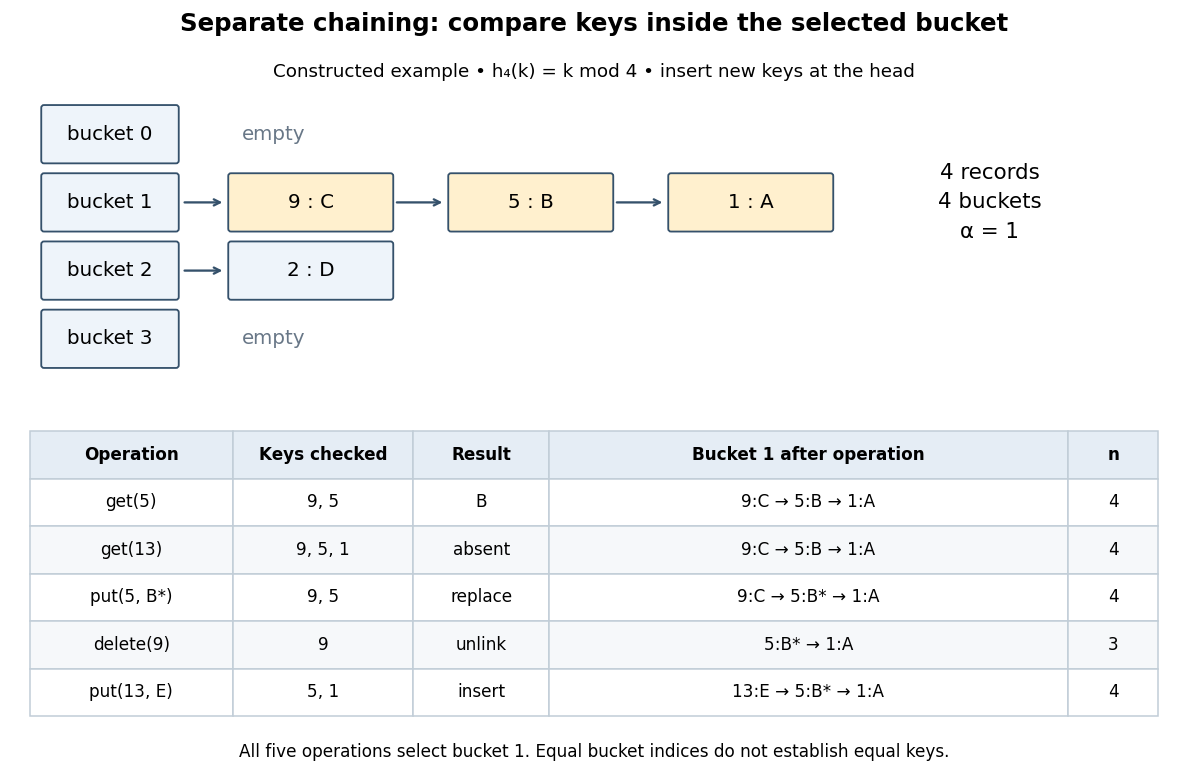
Separate chaining traces lookup, replacement, deletion and insertion through key equality
. Original deterministic model with . The table counts actual keys inspected, not elapsed machine time. Operations occur from top to bottom; only an absent key adds a new record, and the untouched record remains in hash bucket . Details.
get(5) rejects key , accepts key , and returns after two key equality comparisons. get(13) rejects and reports absence after three comparisons. put(5,B*) examines and replaces the value without changing . delete(9) examines just the head record, removes it, and gives . Finally, put(13,E) rejects before inserting the new head record; returns to and the chain is . The successive hash table load factors are . These counts follow from the stipulated chain order; a different insertion policy changes the successful-search counts.For a chain of length , lookup and deletion by key take time complexity in Big O notation. The same applies to
put before any resizing, since replacement semantics require checking for an existing equal key. Head insertion alone is if absence is already known; that is a different precondition. These bounds assume bucket-index hashing, array access, key equality comparisons, allocation and link updates. A long string or large integer can make hashing or comparison depend on its encoded length, so counting record visits alone does not establish constant running time.Under simple uniform hashing, each distinct key's bucket index is an independent random variable with a uniform distribution on a finite set of indices. The keys and query are fixed independently of this random assignment. Then lookup has expected time complexity, where is the hash table load factor; it is expected when stays bounded. These are model assumptions, not an automatic consequence of using a deterministic hash function.[ref]
Lecture 8: Hashing I. 6.006 Introduction to Algorithms, Fall 2011 by Massachusetts Institute of Technology, 6.006 course staff; pp. 4–5, chaining worst case and simple uniform hashing assumption
Here is the short calculation. For an absent query and stored keys , let be the indicator random variable of . The number of records inspected has expected valueby linearity of expectation. For a present fixed query, scanning its entire chain inspects at most itself plus all other colliding records, with expected value ; stopping at the match only decreases this upper bound. Adding constant hashing and bucket access yields expected for either query. The argument needs pairwise collision bounds; it does not require all the indicator random variables to be independent. A universal hash family can provide a related bound by random choice of a hash function for a fixed key set, as explained in that article.
The worst case remains , and an absent query takes comparisons if all records occupy its hash bucket. For instance, all collide under . Separate chaining remains correct, but a sequence of insertions that each checks the existing chain can take quadratic total work. Amortized analysis of resizing does not remove this search cost, and an adaptive choice of keys based on a known hash function is outside the stated simple uniform hashing model.
Splay tree 2026-10-31
A splay tree is a binary search tree whose access operations use splaying to move a selected key to the root through tree rotations. It stores no explicit balance or height information. A single access can take linear time, while the standard operations have logarithmic amortized time complexity. The distinction matters: amortized analysis bounds the total cost of an operation sequence, not the worst cost of every individual operation.[ref]
Self-Adjusting Binary Search Trees by Daniel Sleator and Robert Tarjan. Author-hosted abstract: representation, operations and amortized logarithmic bound