A binary string is a finite word over the alphabet . There are strings of length . Finite binary strings have an effective bijection with natural numbers, so computable enumerability and immunity apply to sets of strings.
A binary string with zeroes and ones is determined by its one-positions, giving possibilities. Sum for and apply the hockey-stick identity. Equivalently, distribute at most ones among the gaps around the zeroes and add a slack count; stars and bars counts nonnegative counts summing to .
A self-delimiting code permits a decoder to identify the end of a code without an external length marker. Encoding a binary word of length by ones, a zero and the word uses bits. This yields an description of a natural number in an incompressibility proof.
For formal languages over the same alphabet, concatenate each word over an alphabet in with each word over an alphabet in . This operation is associative, has identity and absorbing element the empty language.
The formal language containing no words over an alphabet. It differs from the language containing only the empty word, which is a multiplicative identity for concatenation of formal languages.
A Turing machine is an abstract computational model with a finite control, an unbounded tape and a head that reads, writes and moves on the tape.
An instantaneous description records the current control state, head position, and tape contents. For a tape blank outside a finite window, a word records the symbols to the left of the head and from the scanned cell rightward, with unrecorded cells blank. If is empty, the head scans an implicit blank. Extra outer blanks can represent the same infinite tape. The instruction of a Turing machine determines its successor description.
For a deterministic single-tape Turing machine, an instruction reads a state and scanned tape symbol , writes , changes state to , and moves the head one cell left, one cell right, or not at all according to . The state and tape alphabets are finite; an undefined transition halts. A dedicated terminal state can be introduced by directing undefined transitions to it without changing whether computation halts.
Encode the cells immediately left of the head in a reversed positional stack , and the current and right cells in . Quotient and remainder by the alphabet base read and remove cells; multiplication by that base pushes a cell. The resulting local tape transitions are primitive recursive, which makes them directly implementable on Church numerals.
A modular machine of modulus acts on pairs in . Each instruction or has and , and at most one instruction is assigned to each residue pair . The two transition types are and . These finite arithmetic operations can encode a Turing machine; a designated terminal configuration can have a nonrecursive halting set.
A modular machine can be encoded by HNN extensions of . The kernel of has a free basis of a group . Associated-subgroup maps send these basis elements according to the two arithmetic transition types. In the resulting group, membership of in the subgroup generated by and the instruction stable letters is equivalent to . One more HNN extension centralizes that finitely generated subgroup, converting membership to equality and hence to the word problem for a group.
For a modular machine whose is terminal, is the set of configurations whose forward computation reaches exactly , including the zero-step computation there. It may differ from the set of configurations stopping at any terminal configuration. Determinism makes membership invariant along each instruction edge.
In a deterministic computation, every configuration and input symbol determine at most one next configuration.
A reversible computation has an injective transition function, so its preceding configuration can be recovered from its current configuration. Any finite classical computation can be simulated reversibly while retaining enough workspace to uncompute its temporary results.
A reversible circuit is composed of bijective gates. The Toffoli gate is universal for reversible Boolean computation when ancillary bits are available.
A nondeterministic computation may have several possible next configurations and accepts when at least one computation path accepts.
A Boolean operation is a Boolean function taking truth values encoded as bits: means false and means true. These operations supply the concrete two-valued interpretation of a Boolean algebra. A Boolean valuation fixes the inputs; a truth table lists every possible input. With two input bits there are four rows.
The basic logical connectives are logical conjunction (AND, , both true), logical disjunction (OR, , at least one true), exclusive or (XOR, , exactly one true), and logical negation (NOT, , the opposite value). OR is inclusive: it accepts the case where both inputs are true.[ref]
3.1 Propositional Logic. Discrete Mathematics: An Open Introduction (3rd edition) by Oscar Levin; Discrete Mathematics: An Open Introduction, 3rd edition by Oscar Levin, §3.1, Truth Tables: conjunction, disjunction and negation tables
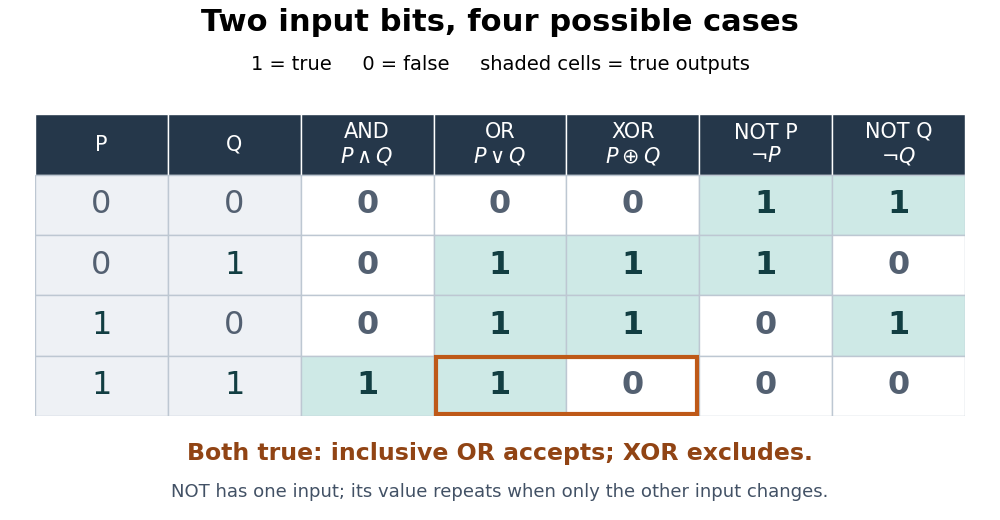
Four input pairs distinguish logical conjunction, inclusive logical disjunction, exclusive or, and logical negation
. Details. For an original program-condition example, let mean “the backup is recent” and mean “the backup is verified”. A rule requiring a recent, verified backup uses logical conjunction; one accepting either qualification uses logical disjunction. A rule flagging a mismatch between the two qualifications uses exclusive or. A recent, verified backup gives : AND and OR accept it, while XOR does not flag it. The last row of the truth table makes this difference explicit.
The same small Boolean operations build larger tests and Boolean circuits. In a programming language, the value of a condition and the procedure for evaluating it both matter. For Boolean operands, Python's
and, or, and not implement these logical connectives. Evaluation proceeds from the left; and skips its right operand if the left is false, and or skips it if the left is true. More generally, and and or return an operand, whereas not returns a Boolean.[ref]Expressions, Python 3.14 language reference. Python 3.14 documentation; Python Language Reference, version 3.14, §6.11 Boolean operations: evaluation order and returned operands
For example, the Python condition
denominator != 0 and numerator / denominator > 2 avoids division by zero because the logical conjunction's second test is evaluated only when the first succeeds. Reversing the tests preserves the abstract truth table for defined operands but can raise a division-by-zero error handled through exception handling. A rewrite involving a side effect must also preserve the needed evaluation behavior.Events turn Boolean operations into operations on sets. For a die with sample space , let be the event “even outcome” and the event “outcome at least four”. At outcome , use the indicator functions and . ThenThus logical conjunction becomes set intersection, logical disjunction becomes set union, exclusive or becomes symmetric difference, and logical negation becomes the complement of a set within . Outcome four satisfies both events, so inclusive logical disjunction includes it and exclusive or excludes it. If the die is fair, these four events have probabilities , , , and , respectively. No assumption of independent events is needed for the set identities; indeed and here are not independent, since .
Exclusive or returns one exactly when its two input bits differ. Its truth table gives , , , and . The identitiesexpress exclusive or using logical conjunction, logical disjunction, and logical negation. The first expression accepts at least one input and then excludes both; the second explicitly lists the two accepted input pairs.
For numerical bits, exclusive or is addition in modular arithmetic modulo two:The binary operation is commutative and associative, because addition modulo two has those properties. It satisfies , , and . These identities explain why a bit can be toggled and restored with the same operation.
On binary strings of equal length, bitwise exclusive or applies the one-bit rule separately at each position. For example,A bit mask of toggles exactly the middle two bits. Applying the mask twice restores the original binary string: each selected bit changes twice, and each unselected bit stays fixed. This positional operation is distinct from taking the exclusive or of the overall truth values of two integers.
For bits , repeated exclusive or computes the parity of the number of ones:An induction proves this: the first bit gives its own parity, and appending a zero preserves it while appending a one changes it. The binary string has three ones, so its parity bit is one. Append that parity bit to obtain , whose six bits have even parity. Flipping the second bit produces and changes the combined exclusive or to one, detecting an error. Flipping the third bit as well produces , with four ones and combined exclusive or zero: an even number of flips can escape this check.
For three inputs, repeated exclusive or means an odd number of true inputs, rather than exactly one: . The “exactly one” description applies to the two-input exclusive or. This distinction matters when translating a requirement that exactly one option be selected into a program condition.
Logical negation exchanges zero and one: and . For a numerical bit , this is ; applying logical negation twice restores . It acts on the entire propositional formula in its scope. Parentheses therefore matter: says that neither condition holds, while also accepts every case where holds. At their values are zero and one.
On a set, logical negation becomes taking a complement in a fixed universal set. In Boolean operations on events, “not even” selects . “Not both even and at least four” selects ; it does not require both qualifications to fail. De Morgan's laws make the scope of these compound negations precise.
De Morgan's laws exchange logical conjunction and logical disjunction when a logical negation moves across them:Here denotes logical equivalence: the two propositional formulas agree under every Boolean valuation.[ref]
3.1 Propositional Logic. Discrete Mathematics: An Open Introduction (3rd edition) by Oscar Levin; Discrete Mathematics: An Open Introduction, 3rd edition by Oscar Levin, §3.1, Logical Equivalence: definition, Example 3.1.3 and De Morgan's Laws box
A complete verification uses the four rows of a truth table. In input order , both sides of the first logical equivalence have output sequence ; both sides of the second have . A proof in words is equally short: failure of “both” means at least one failure, whereas failure of “at least one” means both fail. The differing middle rows explain why simply pushing logical negation inward without changing AND to OR is wrong.
For the events in Boolean operations on events, the corresponding set identities areOne can prove these identities by checking an arbitrary set element : its two membership truth values obey De Morgan's laws. The same reasoning works for any two subsets of a common universal set.
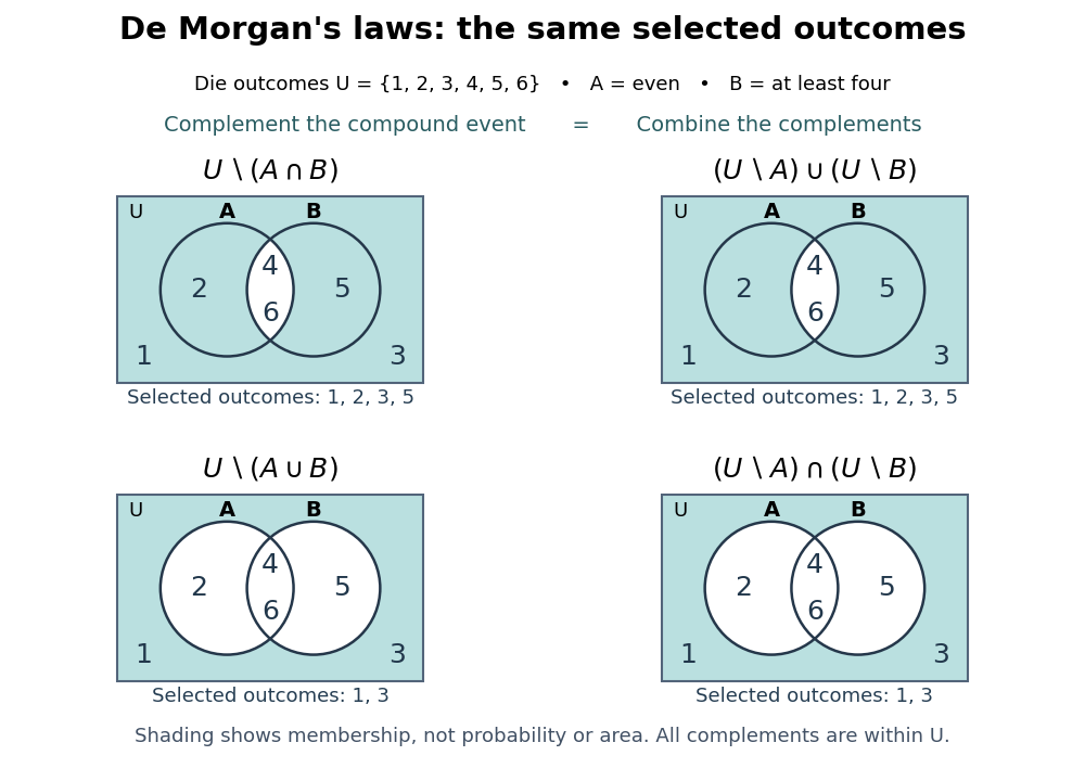
De Morgan's laws shade the same set whether a compound event is complemented first or its component events are complemented first
. Details. For a nested program test, let mean “backup recent”, mean “backup verified”, and mean “manual override authorized”. Rejecting when neither an acceptable backup nor an override is present givesThe transformed condition reads “backup stale or unverified, and no override”. Apply the second of De Morgan's laws at the outside, then the first at the inner logical conjunction. For it rejects; changing only to one makes it accept. With Boolean operands in Python,
not ((recent and verified) or override) and ((not recent) or (not verified)) and (not override) have the same result and inspect the operands in the same order, with the same skipped operands.For a Boolean function of input bits, define its De Morgan dual by complementing every input, applying , and complementing the output:
De Morgan's laws say that the De Morgan dual of logical conjunction is logical disjunction, and conversely. The constant zero Boolean function becomes constant one. This is different from merely negating the output: for AND, output logical negation gives one at , whereas the De Morgan dual gives zero there.
Taking the De Morgan dual twice restores the original Boolean function:Here each input is complemented twice as well. For a Boolean formula built from AND, OR, NOT and constants, its De Morgan dual can therefore be obtained by exchanging AND with OR and zero with one throughout, leaving input names and NOT in place. A structural induction proves the rule: it holds for an input and each constant, De Morgan's laws handle the two binary logical connectives, and double logical negation handles NOT. This symmetry lets one translate a complex test systematically instead of guessing where its failures occur.
Computational complexity theory classifies computational problems by the resources needed to solve them.
Communication complexity studies how much information distributed parties must exchange to compute a function of their separately held inputs. Local computation is free; the resource being counted is communicated bits or qubits, with the allowed shared randomness, quantum entanglement or other correlations specified separately. For a Boolean function , a one-way exact protocol has the receiver output correctly for every input after a single message. One-bit computation using Popescu–Rohrlich boxes shows that this resource measure changes drastically if ideal superquantum boxes are available.
A promise problem consists of disjoint sets of YES and NO instances. An algorithm or verifier must obey its correctness guarantees only on their union. Energy problems with separated thresholds are naturally promise problems because intermediate-energy instances require no prescribed answer.
Quantum complexity theory studies resources needed by quantum circuits and quantum algorithms, including time, workspace, and quantum query complexity. Its models specify which input oracles and gate implementations are available; counting oracle calls is different from counting all elementary gates.
BQP is the class of promise problems decided by uniform polynomial-size quantum circuits with bounded error. Completeness and soundness are conventional; BQP error reduction shows that other fixed separated thresholds give the same class.
Independent runs of a BQP algorithm with fresh ancilla qubits can be combined by a classical threshold rule. If completeness exceeds soundness by , a Hoeffding inequality bounds the error after runs by . Polynomial repetition handles inverse-polynomial gaps. This does not automatically preserve the restricted gate and measurement rules of a stoquastic circuit.
A quantum witness is a polynomial-size quantum state supplied to a verifier as evidence for a YES instance. The verifier fixes its own ancilla qubits independently. Pure quantum witnesses suffice when maximizing a linear acceptance functional on density operators. Quantum witnesses are not generally restricted to basis vectors or product states.
StoqMA is a restricted quantum-verifier class using stoquastic circuits and polynomial-size quantum witnesses. A YES instance has a quantum witness accepted with probability at least ; on a NO instance every quantum witness has acceptance at most , with an inverse-polynomial gap . An optimal quantum witness can be chosen with nonnegative amplitudes, since the witness acceptance operator is entrywise nonnegative. The quantum witness is generally a superposition, rather than a computational basis vector. The stoquastic acceptance floor explains the lower limit for a nontrivial soundness promise.
QMA is the class of promise problems with a polynomial-size quantum witness checked by a uniform polynomial-size quantum circuit. YES instances have an accepting witness with probability at least ; NO instances have acceptance at most for every witness, including mixed states. The verifier's acceptance is linear in the witness density operator. Inverse-polynomial or exponentially small error can be obtained through QMA error reduction.
For quantum witness embedding , verifier unitary and accepting projector , the witness acceptance operator is the positive contraction . The maximum acceptance over normalized quantum witnesses is by the Rayleigh quotient. Restricting to basis quantum witnesses only tests its diagonal entries and need not find that maximum.
For a positive witness acceptance operator on dimension , large trace powers approximate its largest eigenvalue. With an -qubit QMA quantum witness and , the usual NO instances give and YES instances give a value above . A closed product-index expansion computes the trace by recomputation with polynomial storage, avoiding logarithms and roots in a real-arithmetic implementation.
Starting from completeness and soundness , run an odd number of parallel copies and take majority. The QMA parallel repetition with entangled witnesses argument proves soundness for arbitrary repeated witnesses. Exponential Markov's inequality gives majority error at most . Hence copies suffice for error , with polynomial overhead when the target error is inverse-polynomial or exponentially small in input length.
Independent verifier circuits on witness registers induce a threshold acceptance effect built from tensor products of and , where is the quantum verifier acceptance operator. In a product eigenbasis of , the effect's eigenvalues are threshold probabilities for independent Bernoulli random variables with parameters given by the selected eigenvalues of . Bounding every parameter on a NO instance bounds the effect's operator norm, even if the actual submitted witness is entangled. Independence is used only for the spectral calculation, not assumed for the witness.
A verifier with clean ancillas and a designated output measurement induces an effect on the witness register. Its acceptance probability is , and the largest possible acceptance is . Spectral bounds on make the soundness quantifier over all witnesses, including entangled repeated witnesses, explicit.
The quantum query complexity of a task counts uses of an input oracle by a quantum circuit, for a specified success probability. Known gates and workspace operations are not counted as oracle queries, although they contribute to the circuit's full runtime. An efficient query bound therefore need not, by itself, be an efficient gate bound.
After input-bit queries, every probability amplitude is a polynomial of degree at most , because the bit-query matrix entries are affine in the input bits. An acceptance probability is a sum of squared absolute amplitudes and has polynomial degree at most . Multilinear reduction on the Boolean cube does not increase degree. Exact acceptance therefore implies . For bounded error the acceptance polynomial only approximates the Boolean function; its exact representing degree is not the relevant bound.
The least worst-case number of input-oracle calls made by a quantum circuit that computes a Boolean function with zero error on every input. Known unitary gates and classical processing do not count toward this quantity; their runtime is a separate cost.
One exact parity query determines whether the first two bits agree. If they agree, a second query reads one of them; otherwise it reads the third bit. Those values respectively determine the three-bit majority function. The matching lower bound follows from its degree-three multilinear polynomial.
Given a function with an -bit output, accessed through the unitary operator , quantum collision finding asks for distinct inputs with equal outputs. Here is bitwise exclusive or on the -bit answer quantum register. The distinctness requirement excludes the uninformative pair . For a two-to-one function on inputs, Grover search algorithm methods yield a cube-root quantum query complexity, despite a square-root cost for finding a partner of just one preselected input.
Query a known set of inputs and store its output table. If no function collision occurs there, each of its distinct outputs has exactly one partner in the complement, for a two-to-one function. A compute-phase-uncompute construction marks those partners using two function queries and reversible table comparison. Known-subset Grover search then uses such phase queries. Including table preparation and a final verification query givesChoosing balances both terms and gives . The Grover rotation angle rounding bound gives success tending to one. This is a query bound; it does not make reversible table lookup free in a gate or physical-memory cost model.
A decision tree represents a deterministic computation of a known Boolean function by inspecting input bits. Each internal vertex of its binary tree names a coordinate to query, its two outgoing edges carry answers 0 and 1, and each leaf carries the output 0 or 1. Starting at the root of a tree, read the named bit, follow its answer edge, and repeat until a leaf is reached. Correctness requires the leaf's label to equal for every input .[ref]
Complexity Measures and Decision Tree Complexity: A Survey by Harry Buhrman and Ronald de Wolf. Buhrman and de Wolf, Complexity Measures and Decision Tree Complexity: A Survey, section 3.1, manuscript p. 5: deterministic trees and D(f)
The next coordinate, or the decision to stop, can depend on earlier answers: this is adaptive querying. The same input always follows the same graph path; adaptivity does not require randomness. A correct leaf must have the same output for every completion of the observed bits. Thus a decision tree can stop as soon as the observations form a query certificate. Querying an already known coordinate adds no information, so we use decision trees without repeated coordinates on a graph path; an efficient tree also removes queries made after the output is already forced.
The motivation is exact computation with shortcuts. If inspecting an input entry is expensive, the question is how much of the input must actually be read. The decision-tree query cost counts these inspections, while local calculations on known values are free in this model; this cost need not equal an implementation's time complexity. Here the Boolean function is specified in advance and must be computed exactly on every input. Decision tree learning instead fits a predictor from data, with a different objective.
Three votes give a small but revealing majority function:Our decision tree queries , then . If these bits agree, return their common value: two equal votes already force the majority function. If they disagree, query and return its value. The first two queries have a fixed order, but whether a third query occurs is adaptive.
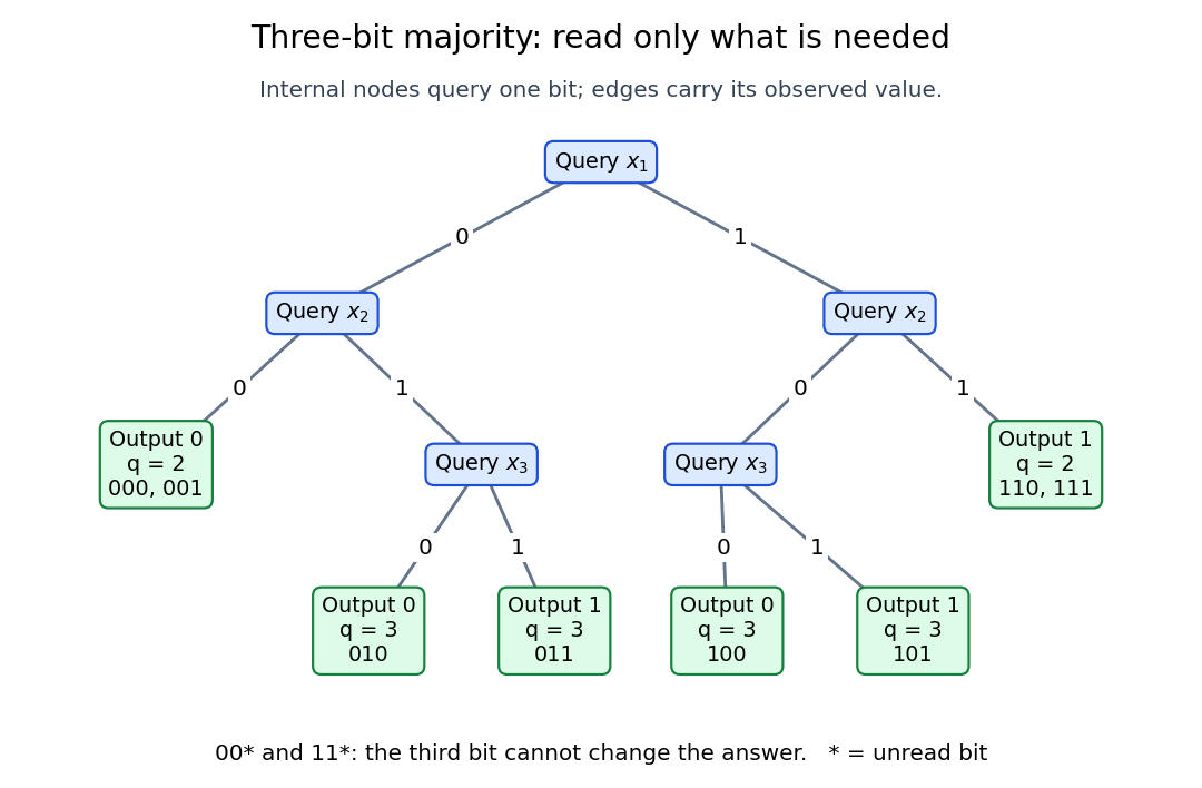
Each internal label in the diagram names the next bit to inspect. Each leaf lists its output, decision-tree query cost , and compatible inputs; an asterisk denotes an unread bit. The two shallow leaves each cover two inputs, while each deeper leaf covers one. Reading every bit would also compute the majority function, but would miss these exact shortcuts.
All eight inputs give the following exhaustive check. The parity column is the parity of , computed by exclusive or; its decision-tree query cost is justified under parity lower bound for Boolean queries.
The worst inputs for this decision tree are , exactly those with . Its actual depth is three. Every exact decision tree for this majority function has depth at least three: after the first query, an adversary can answer the second distinct query with the opposite bit, leaving the last bit decisive. Consequently its optimal decision-tree depth is , even though some inputs finish sooner. Every input has a two-bit query certificate, namely two agreeing votes; locating those votes can require a third query. This separates having a short query certificate from finding one.
For three bits, the Boolean function outputs one when is odd, where denotes exclusive or. Unlike the three-bit majority decision tree, an exact decision tree computing parity must inspect all three bits on every input. If any coordinate is unread, two completions differing only at that coordinate follow the same observed graph path but have opposite parity. A single leaf cannot correctly label both.
The same argument works for bits: parity needs all queries on every input, whatever their order. Thus its decision-tree depth is , its expected query cost is for every input probability distribution, and each coordinate revealment is one. The algorithm remains required to be correct on the whole Boolean cube, even if the chosen probability distribution assigns some inputs zero probability; a promise restricting permitted inputs would be a different computational problem.
For a particular decision tree , its decision-tree query cost is the number of queries along the graph path followed by input . Its actual tree depth isThe query vertices count as operations; each is followed by one answer edge. Thus a leaf reached after queries has graph path length , and a tree consisting only of an output leaf has depth zero. With no repeated coordinates, . The decision-tree depth minimizes over all correct decision trees for ; measures the chosen algorithm, while measures the Boolean function.
Choose an input probability distribution and let have that distribution. Then is a random variable even when the decision tree is deterministic. Its probability mass function describes how often each path length occurs, and its expected value is the expected query cost. None of these quantities changes the actual maximum depth of .
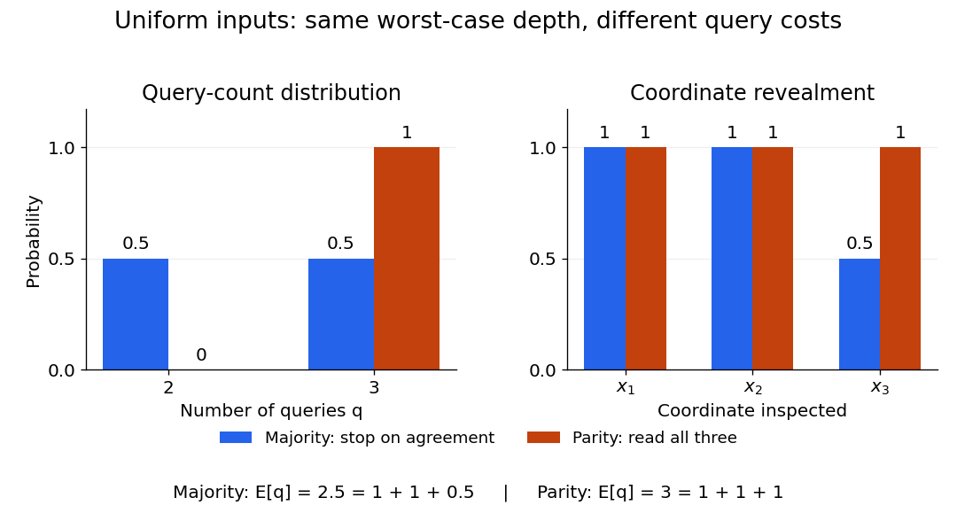
Uniform three-bit inputs: query-count distributions and coordinate revealment for majority and parity
. Details. The left panel aggregates the eight inputs from the three-bit majority decision tree: four cost two queries and four cost three. Parity always costs three. The right panel asks a different question, which coordinates are inspected: the majority function algorithm always queries coordinates 1 and 2, but queries coordinate 3 only on disagreements. These are probabilities of inspection, not probabilities that a bit equals one.
For a fixed decision tree and input probability distribution , its expected query cost isUnder the discrete uniform distribution on the eight three-bit inputs, the three-bit majority decision tree hasThis is an exact average, not a fractional query made during one execution. It is also optimal among exact deterministic decision trees under this discrete uniform distribution: one observed bit never determines the majority function; whichever two distinct coordinates are inspected first, their values disagree with probability , forcing a third query. In comparison, querying all three bits unconditionally has the same actual depth three but expected query cost three.
For an arbitrary input probability distribution, the same fixed three-bit majority decision tree gives . For three independent random variables, each a Bernoulli random variable with common one-probability , this becomes ; the value depends on . Averaging over inputs should also be distinguished from averaging over an algorithm's internal random choices at a fixed input.[ref]
The coordinate revealment of coordinate for a decision tree under input probability distribution isIt depends on the chosen decision tree and the probability distribution, not just on the Boolean function. Since no coordinate is queried twice on a graph path, indicator functions giveThe second equality uses linearity of expectation; it does not require independence of random variables or a product measure. The cited paper defines these inspection probabilities and their sum for product measures; the displayed indicator function argument extends the identity to any input probability distribution.[ref]
For the three-bit majority decision tree under the discrete uniform distribution, , whose sum is . Reading coordinate 3 first, then coordinate 1, and stopping on agreement gives the same majority function, depth and expected query cost, but coordinate revealments . The asymmetry belongs to the chosen query order. Parity gives for every exact decision tree without repeated queries. If repeated queries were charged, inspection probabilities would count distinct coordinates; total query count would instead require expected multiplicities.
The decision-tree depth of a Boolean function is the smallest possible maximum number of input coordinates queried along any root-to-leaf graph path of a decision tree computing :The actual depth of a particular decision tree can exceed this optimum. A constant function admits a depth-zero tree even though an inefficient algorithm could inspect its entire input before returning that constant. Expected query cost and coordinate revealment additionally require an input probability distribution; does not. The three-bit majority decision tree and three-bit parity both have optimal decision-tree depth three, although only the former has the two-query shortcuts described above.
A query certificate fixes some input coordinates to their values in a chosen input and must force the output for every completion. The smallest such size is ; maximizing over accepted or rejected inputs gives or , and maximizing both gives . A one-sided maximum over an empty output class is defined as zero. This is query certificate complexity, distinct from polynomial verification of a witness in NP.
For a Boolean function and a chosen input , a set of coordinates is a query certificate if every agreeing with on has . It fixes actual input bits rather than supplying an independently guessed certificate to an NP verifier. Minimizing its size at each input and then maximizing gives query certificate complexity.
A Boolean function is evasive when every deterministic decision tree computing it has a worst-case path that queries all input bits. The alternating-sum criterion for decision-tree evasiveness is one sufficient method for proving this lower bound.
A leaf reached before all input bits are queried leaves at least one coordinate free. Flipping that coordinate pairs its inputs with opposite alternating signs and equal output. Thus every such leaf contributes zero. If the total alternating sum is nonzero, a depth below is impossible.
To prove that a threshold function requires every input bit in the worst case, an adversary answers queries while keeping completions on both sides of the threshold possible. If this remains true until the final unqueried bit, every decision tree has depth equal to the number of variables.
A decision problem asks for one of two answers, conventionally encoded as zero and one. Equivalently, it asks whether an input belongs to a formal language.
A search problem asks for a witness satisfying a specified relation rather than only whether one exists.
A search-to-decision reduction reconstructs a witness by making queries that only decide whether a suitable witness exists.
A complexity class is a collection of computational problems sharing specified resource bounds and a computational model.
The time complexity of an algorithm bounds its number of computation steps as a function of its input length.
Specify both the size parameter and the operations counted. For binary search, take to be the number of array entries and count a three-way comparison of the target with one entry as one operation. Code using separate equality and less-than tests may perform two primitive tests per inspected entry; this changes a constant factor. The input size in bits is a different parameter when entries have variable-length representations.
Worst-case time complexity maximizes the count over permitted inputs of size . An absent target forces comparisons in linear search. For binary search, the worst-case count is for , attained by a target larger than every entry. Both have a best case of one comparison when the first inspected entry matches.
In Big O notation, the worst-case bounds are and respectively. Here means that fixed constants exist with for all . It is an upper bound, so a logarithmic count is also ; the sharper bound communicates its scaling better. The base of the logarithm changes only a constant factor.
For , linear search can require comparisons, whereas binary search needs at most , since . Doubling adds just one to the worst-case binary search count. These are operation counts, not measured machine runtimes. Translating them into logarithmic execution time assumes constant-cost indexed access, comparison and index arithmetic. Long entries can make comparison expensive; a linked list does not provide constant-cost access to an arbitrary middle index. Building or sorting the array is additional work: merge sort can provide order for many subsequent searches, but its cost belongs in the analysis too.
An algorithm has pseudo-polynomial time when its running time is bounded by a polynomial in the numerical magnitudes of input quantities, rather than necessarily in their encoded length. The dynamic programming table for the 0-1 knapsack problem uses arithmetic operations for items and capacity . A binary numeral system encoding needs only bits for that capacity, so the table bound can be exponential in the number of capacity bits. This distinction does not claim that every input requires exponential work.
Bounds the total cost of a sequence of operations, rather than a probability-weighted average. If a nonnegative potential assigns stored credit to states, define . Then . Starting with zero potential, constant amortized costs imply linear total cost.
// Destination: computer-science.bigb
An algorithm runs in polynomial time when its running time is at most for some constant , where is the input length.
An algorithm runs in polynomial time if its worst-case running time is bounded by a fixed polynomial in the input length. Arithmetic with fixed-degree algebraic numbers also needs polynomial bit cost when used in such a guarantee. The Edmonds–Karp algorithm and the method of conditional probabilities with efficiently computable clause expectations are examples.
A language in P to which every P language has a logspace many-one reduction. The reduction strength matters: using arbitrary polynomial-time reductions instead would make completeness trivial for nontrivial P decision problems.
is the class of decision problems whose positive instances have polynomial-length certificates verifiable in polynomial time. Equivalently, it is polynomial time on a nondeterministic computation.
A certificate for a positive instance is a polynomial-length string that makes a polynomial-time verifier accept that instance.
The space complexity of an algorithm bounds the amount of working memory it uses as a function of input length.
An algorithm uses polynomial space if its working memory is bounded by a fixed polynomial in the input length. Exponentially many possibilities can still be searched when each candidate and the search counter need polynomial space and storage is reused. The decision problems with deterministic polynomial-space algorithms form PSPACE.
Languages accepted by Nondeterministic Turing machines using work space on every computation path, with acceptance defined by existence of an accepting path. Bounded-space loops do not prevent the reachability interpretation in the finite configuration graph.
Reachability within steps can be tested by enumerating a midpoint and recursively testing two half-paths. Configurations have bits and recursion depth , yielding deterministic space . The space-bound discovery by exit reachability permits this simulation without assuming that the supplied function is constructible.
For a bounded-space machine, start with a logarithmic work budget and test accepting reachability and reachability of a transition leaving the budget. Accept if acceptance is found, double the budget if an exit is reachable, and otherwise reject. If all paths use at most space, doubling stops at . Each budget test uses the Savitch theorem recursion and the storage is reused. The method discovers a sufficient bound without computing .
Languages decidable by deterministic Turing machines using work-tape cells with a read-only input. Input-head addresses take bits, while the input itself is not charged to work space. The definition does not require the bound to be computed by the deciding machine.
PSPACE consists of decision problems solvable using a polynomial amount of work space. Running time may be exponential. Enumerating all polynomial-length relation encodings and reusing working storage preserves this bound, as does complementation. In particular fixed-sentence second-order logic model checking lies in PSPACE.
A polynomial-register real-arithmetic computation stores polynomially many real numbers and may use arbitrarily many additions, subtractions and multiplications, with comparison tests for decisions. Register count does not bound precision or time. Fixed gate constants or sufficiently accurate computable approximations must be specified. This resource model is distinct from ordinary bit-cost computation.
A decision problem is NL-complete when it belongs to NL and every problem in NL reduces to it by a deterministic logarithmic-space many-one reduction.
Decide whether a directed graph has a nonempty directed cycle; self-loops count. This problem is NL-complete. Membership guesses a returning walk of at most the vertex count. For hardness, layer a reachability instance into layers with wait arcs, then add only the backward edge from the target in the last layer to the source in the first. The otherwise acyclic layering has a cycle exactly when the original target is reachable. Zero-length paths must not be treated as cycles.
The directed graph reachability problem asks whether a directed graph contains a directed path from a specified vertex to a specified vertex . It is NL-complete.
The configuration graph of a machine on a fixed input has one vertex for each machine configuration and a directed edge for each valid computation step.
consists of complements of languages in NL.
The Immerman–Szelepcsényi theorem states that . Its proof uses inductive counting of reachable configurations.
Inductive counting certifies the number of vertices reachable within successively larger path-length bounds. Knowing the exact earlier count lets a logarithmic-space nondeterministic machine certify that no reachable predecessor has been omitted.
A polynomial-time reduction transforms instances of one computational problem into instances of another using a polynomial-time algorithm.
A polynomial-time many-one reduction from a decision problem to a decision problem is a polynomial-time computable function satisfying exactly when .
A total mapping with exactly when , computed by a deterministic logarithmic-work-space transducer with read-only input and write-only output. Such reductions compose, and are used for NL-completeness and P-completeness. The output can be polynomially larger than the work storage.
Given subsets of a finite universe, the decision problem asks whether at most of them cover the universe. It is NP-complete. If , existence of a cover by at most subsets is equivalent to existence of a cover by exactly , by adding unused subsets. The promise that every element occurs in some subset loses no hardness: an uncovered element can be detected in polynomial time and mapped to a fixed negative instance.
// Target: mathematical-optimization.bigb
Assume and . Construct a two-player game with row for and columns . Column pays both players one; column pays when , and otherwise. There is a Nash equilibrium whose row player's support of a mixed strategy has size exactly when rows cover the universe. A uniform mixture on a cover makes column a best response. Conversely, if some element is uncovered by the support, the column player's best responses are uncovered elements and the row player's current payoff is zero. The union promise provides a profitable row deviation. Without the union promise the equivalence is false: a globally uncovered element is a best response against every row mixture.
// Target: mathematical-optimization.bigb
Articles were limited to the first 100 out of 180 total.
Articles by others on the same topic



Theoretical computer science is a branch of computer science that focuses on the mathematical and abstract foundations of computing. It encompasses a variety of topics and concepts that explore the capabilities, limitations, and behavior of computational systems. Some of the key areas within theoretical computer science include: 1. **Algorithms and Complexity**: This area studies the efficiency of algorithms and classifies problems based on their computational complexity. It explores concepts such as P versus NP, NP-completeness, and various complexity classes (e.g.