In 1924–1925, Walther Bothe and Hans Geiger tested event-level Compton scattering correlations against the statistical conservation proposed by BKS theory.[ref]
The Coincidence Method by Walther Bothe. The coincidence method, pp. 271–273
Needle Geiger counters shared a wall. X-rays passed beside it through hydrogen; recoil Electrons registered in one counter and scattered photons triggered Electron release in the other. Photographic records resolved approximately .[ref]
The Coincidence Method by Walther Bothe. p. 272: apparatus and timing
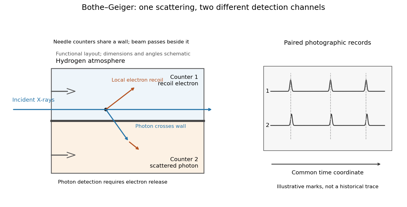
Two detection channels in the Bothe-Geiger coincidence experiment
. Original functional schematic based on Bothe's account; dimensions, angles and trace marks are illustrative. The common wall separates the counter regions; the direct beam avoids it. The drawing specifies neither wall material nor chamber shape. Photon detection requires Electron release. Both records share a time coordinate. Details.
The coincidence excess matched paired-emission expectations. Bothe distinguishes a later directional test from this timing experiment.[ref]
The two channels have different physical roles. The first responds to the local recoil Electron's ionization. The second converts a scattered photon into an Electron response, as in the photoelectric effect. A large counter signal is an amplified indication of an interaction, not a direct measurement of the incoming photon's energy. The detection efficiency and accepted directions determine how many genuine partners can be seen. Consequently, failure to record every partner is compatible with paired production.
The relevant distinction is between an average balance and a balance in each event. For an initially stationary free Electron, Compton recoil kinematics givesHere are incident and scattered photon energies, is recoil kinetic energy, and is Electron momentum. These are paired constraints, not just equations between averages over unrelated detections. Summing correctly paired events preserves the equations; throwing away the pair identities loses information. Two samples can have identical separate energy distributions while differing in their joint probability distribution.
The experiment therefore supplied evidence for the event association required by photon recoil, rather than weighing both outgoing energies in every event. A statistically established excess above accidental coincidences matters; one near-simultaneous pair cannot establish the association. It also cannot by itself settle every question about wave-particle duality.
Preparation, readout and background checks address different failure modes. The direct beam must avoid the second counter, and the counter boundary must prevent a recoil Electron from masquerading as its own photon partner. Separate-channel rates constrain accidental coincidences; common disturbances or electrical coupling could instead create a correlated instrumental background. A useful diagnostic is to displace one record in time: under a stationary process assumption, unrelated-pair expectations persist while prompt partners separate. This is the explanatory control modeled below, not an assertion that Bothe performed that particular record-shifting procedure. A background estimate and a statistical comparison are essential to the inference.
The existing coincidence circuit article explains electronic selection, and accidental coincidence derives the accepted-window background. Here pairing can be understood directly from the two recorded time sequences, without imposing a modern detector trigger on the historical readout.
A photon-recoil lag correlation asks how often a photon record occurs at a specified time displacement from an Electron record. Let be observed separate-channel rates, the rate of detected genuine pairs before a timing cut, and their normalized timing probability density function. For an original dilute, stationary model with observation time , neglecting end effects and detector dead time, the expected pair density isThis counts all pairs of records, rather than at most one detector trigger per Electron. It uses independent unrelated detections for the flat term and an added same-event contribution. A normal distribution for timing spread is a chosen approximation, not a claim about the historical instrument. Intrinsic emission delay, counter response and readout uncertainty can all affect the observed probability density function.
Define the accepted lag interval by : is its full width. Integrating the flat baseline gives the existing accidental coincidence expectation . The additional area is . Moving a window of the same full width away from the peak tests the baseline under the model's stationarity assumption. It does not remove correlated instrumental backgrounds or changing rates automatically.
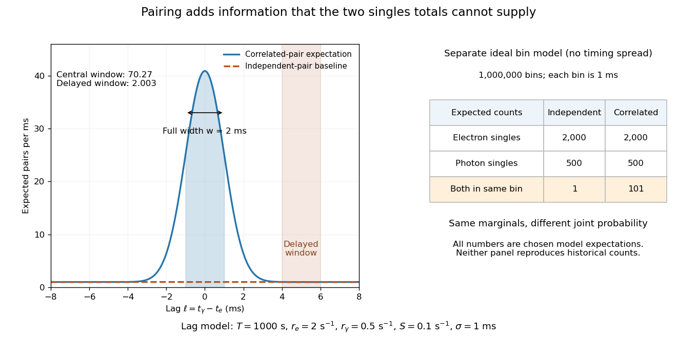
Lag-dependent pairs and a joint probability distribution carry information absent from singles totals
. Original chosen models, not historical counts or fitted data. Left: a normalized normal distribution of genuine-pair lags with standard deviation is added to an independent-pair baseline. Shaded intervals have full width , centered at zero and . Right: a separate exact ideal-bin model ignores timing spread; the two populations have identical singles expectations but different joint expectations. Details.
For the lag model, choose , , , and timing standard deviation . A full width gives expected accidental coincidences and accepted genuine pairs, using the error function. The total is approximately , whereas the displaced interval from to has approximately expected pairs. A finite sample fluctuates around these expectations; these values are not measured counts or a significance calculation.
The right panel isolates the information lost by retaining singles totals alone. In a separate idealized model, stipulate independent bins, with Bernoulli distribution indicators for Electron and photon detection in a bin. Set and . Independence predicts , hence one expected double detection. Alternatively chooseThese nonnegative probabilities sum to one and preserve both marginal probabilities, yet predict double detections in expectation. Their covariance is . This is an exact joint probability distribution illustrating pairing; it does not model the timing spread in the left panel or reconstruct either historical hypothesis quantitatively. Its lesson is why two singles totals cannot decide whether the observed events share a cause.
Articles by others on the same topic
There are currently no matching articles.