X-rays are high-frequency electromagnetic radiation, conventionally with wavelengths of roughly to . The precise wavelength convention varies with context. Hot accreting gas and energetic electronic processes can emit X-rays, whose short wavelengths make them useful probes of compact objects and electron shells.
For a photon, , where is the Planck constant and is the speed of light. As a calculated example, gives , using . The same wavelength can describe different production mechanisms: bremsstrahlung produces a continuous frequency spectrum, whereas Characteristic X-rays arise from discrete electronic changes in chemical atoms. Measuring transmitted X-rays gives radiography; measuring their frequency spectrum gives spectroscopy.
Wilhelm Conrad Röntgen's 1895 first communication describes an induction coil driving an evacuated gas-discharge tube, enclosed in black cardboard in darkness. A paper screen coated with barium platinocyanide showed fluorescence even with its uncoated side facing the tube, visible two metres away. The covering excluded ordinary illumination.[ref]
On a New Kind of Rays by Wilhelm Conrad Röntgen. Röntgen, On a New Kind of Rays, §§1–2; inspected reprint p. 153
He interposed materials: a thousand-page book transmitted; lead was practically opaque. A stepped stack of foil produced a photographic plate record. Different materials were not equivalent at equal density and thickness. Photographic plates checked visual observations while remaining covered against ordinary illumination.[ref]
On a New Kind of Rays by Wilhelm Conrad Röntgen. First communication, §§2–6; reprint pp. 153–154: absorption tests and photographic controls
Section 14 lists photographs of hand bones, wire on a bobbin, boxed weights, an enclosed compass, and a lead-painted door. It does not identify the hand's owner. Magnetic deflection moved the cathode ray impact point and thus the source, without bending the emerging X-rays. Their nature remained unsettled.[ref]
On a New Kind of Rays by Wilhelm Conrad Röntgen. First communication, §§11–14 and 17; reprint pp. 156–157
The observations belong to 1895; the contemporary English translation appeared in Nature on 23 January 1896.[ref]
On a New Kind of Rays by Wilhelm Conrad Röntgen. Catalogue, On a new kind of rays: notes identify the Nature translation and its publication date
The experimental logic separates production, transmission and detection. A visibly opaque covering can transmit X-rays; fluorescence then converts deposited energy into visible light. A shadow measures a difference between paths through an object, rather than a direct view of its surface. Neither a screen's brightness nor photographic darkness alone measures an absolute X-ray energy or establishes the X-ray attenuation law below.In 1924–1925, Walther Bothe and Hans Geiger tested event-level Compton scattering correlations against the statistical conservation proposed by BKS theory.[ref]
The Coincidence Method by Walther Bothe. The coincidence method, pp. 271–273
Needle Geiger counters shared a wall. X-rays passed beside it through hydrogen; recoil electrons registered in one counter and scattered photons triggered electron release in the other. Photographic records resolved approximately .[ref]
The Coincidence Method by Walther Bothe. p. 272: apparatus and timing
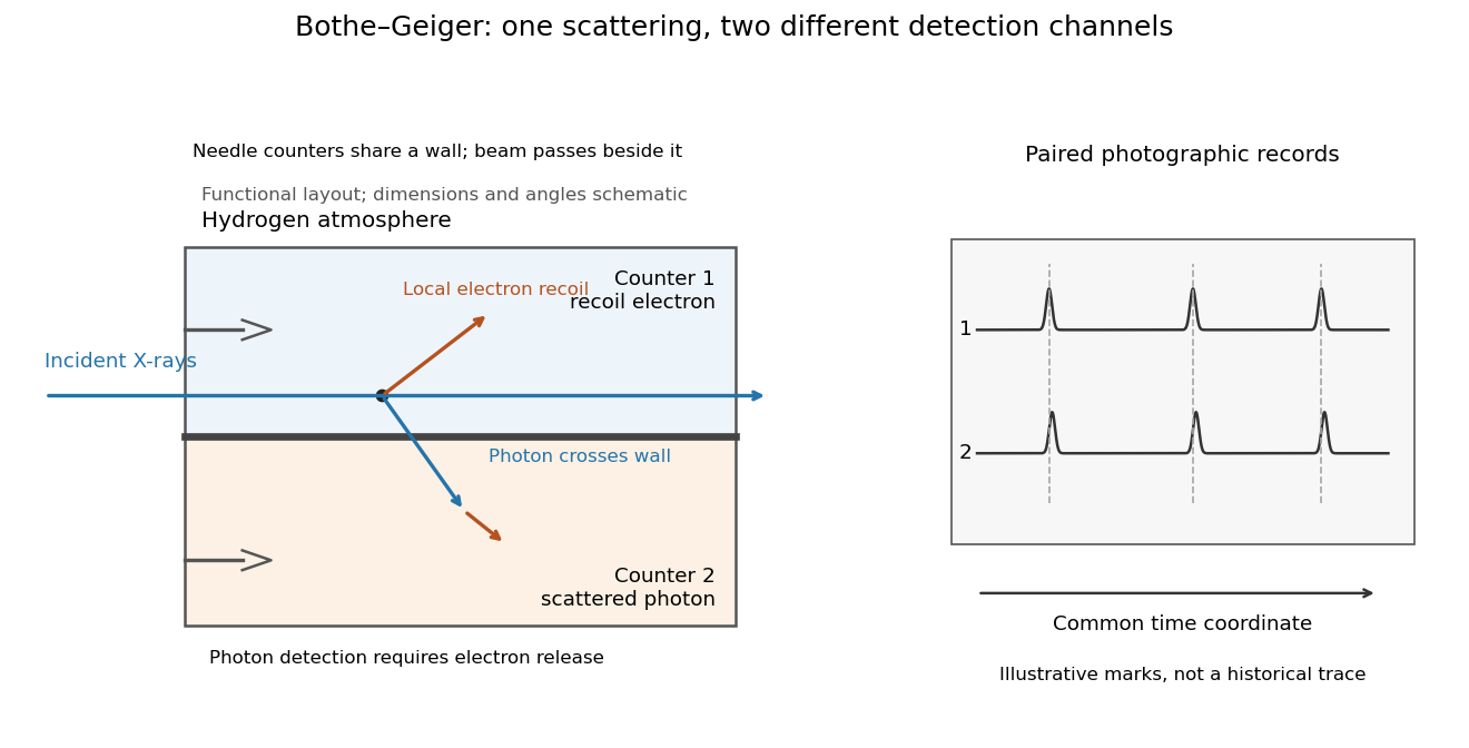
Two detection channels in the Bothe-Geiger coincidence experiment
. Original functional schematic based on Bothe's account; dimensions, angles and trace marks are illustrative. The common wall separates the counter regions; the direct beam avoids it. The drawing specifies neither wall material nor chamber shape. Photon detection requires electron release. Both records share a time coordinate. Details.The coincidence excess matched paired-emission expectations. Bothe distinguishes a later directional test from this timing experiment.[ref]
The two channels have different physical roles. The first responds to the local recoil electron's ionization. The second converts a scattered photon into an electron response, as in the photoelectric effect. A large counter signal is an amplified indication of an interaction, not a direct measurement of the incoming photon's energy. The detection efficiency and accepted directions determine how many genuine partners can be seen. Consequently, failure to record every partner is compatible with paired production.
The relevant distinction is between an average balance and a balance in each event. For an initially stationary free electron, Compton recoil kinematics givesHere are incident and scattered photon energies, is recoil kinetic energy, and is electron momentum. These are paired constraints, not just equations between averages over unrelated detections. Summing correctly paired events preserves the equations; throwing away the pair identities loses information. Two samples can have identical separate energy distributions while differing in their joint probability distribution.
The experiment therefore supplied evidence for the event association required by photon recoil, rather than weighing both outgoing energies in every event. A statistically established excess above accidental coincidences matters; one near-simultaneous pair cannot establish the association. It also cannot by itself settle every question about wave-particle duality.
Preparation, readout and background checks address different failure modes. The direct beam must avoid the second counter, and the counter boundary must prevent a recoil electron from masquerading as its own photon partner. Separate-channel rates constrain accidental coincidences; common disturbances or electrical coupling could instead create a correlated instrumental background. A useful diagnostic is to displace one record in time: under a stationary process assumption, unrelated-pair expectations persist while prompt partners separate. This is the explanatory control modeled below, not an assertion that Bothe performed that particular record-shifting procedure. A background estimate and a statistical comparison are essential to the inference.
The existing coincidence circuit article explains electronic selection, and accidental coincidence derives the accepted-window background. Here pairing can be understood directly from the two recorded time sequences, without imposing a modern detector trigger on the historical readout.
A photon-recoil lag correlation asks how often a photon record occurs at a specified time displacement from an electron record. Let be observed separate-channel rates, the rate of detected genuine pairs before a timing cut, and their normalized timing probability density function. For an original dilute, stationary model with observation time , neglecting end effects and detector dead time, the expected pair density isThis counts all pairs of records, rather than at most one detector trigger per electron. It uses independent unrelated detections for the flat term and an added same-event contribution. A normal distribution for timing spread is a chosen approximation, not a claim about the historical instrument. Intrinsic emission delay, counter response and readout uncertainty can all affect the observed probability density function.
Define the accepted lag interval by : is its full width. Integrating the flat baseline gives the existing accidental coincidence expectation . The additional area is . Moving a window of the same full width away from the peak tests the baseline under the model's stationarity assumption. It does not remove correlated instrumental backgrounds or changing rates automatically.
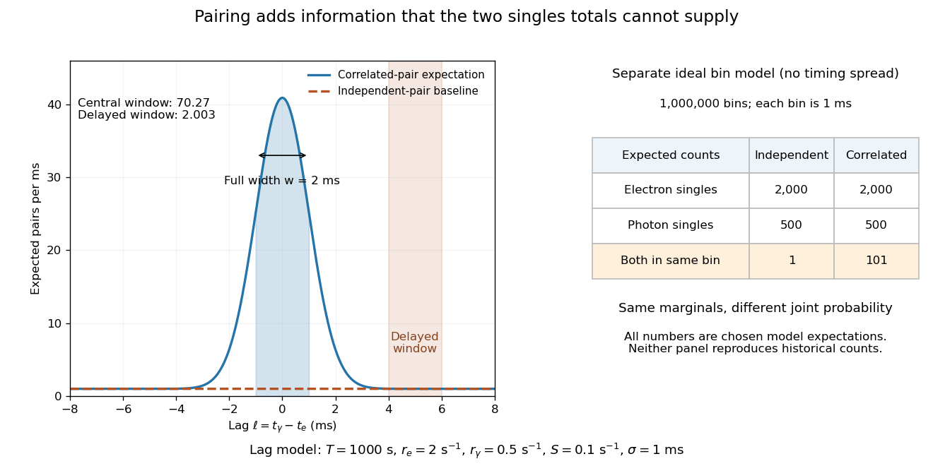
Lag-dependent pairs and a joint probability distribution carry information absent from singles totals
. Original chosen models, not historical counts or fitted data. Left: a normalized normal distribution of genuine-pair lags with standard deviation is added to an independent-pair baseline. Shaded intervals have full width , centered at zero and . Right: a separate exact ideal-bin model ignores timing spread; the two populations have identical singles expectations but different joint expectations. Details.For the lag model, choose , , , and timing standard deviation . A full width gives expected accidental coincidences and accepted genuine pairs, using the error function. The total is approximately , whereas the displaced interval from to has approximately expected pairs. A finite sample fluctuates around these expectations; these values are not measured counts or a significance calculation.
The right panel isolates the information lost by retaining singles totals alone. In a separate idealized model, stipulate independent bins, with Bernoulli distribution indicators for electron and photon detection in a bin. Set and . Independence predicts , hence one expected double detection. Alternatively chooseThese nonnegative probabilities sum to one and preserve both marginal probabilities, yet predict double detections in expectation. Their covariance is . This is an exact joint probability distribution illustrating pairing; it does not model the timing spread in the left panel or reconstruct either historical hypothesis quantitatively. Its lesson is why two singles totals cannot decide whether the observed events share a cause.
An X-ray tube accelerates electrons from a negative cathode to a positive target anode. A heated cathode supplies electrons by thermionic emission; the evacuated envelope limits collisions before the target. This differs from the gas-discharge tube in the Röntgen X-ray discovery experiment.[ref]
Chapter 5: X-Ray Production (teaching slides) by K. P. Maher. Diagnostic Radiology Physics: A Handbook for Teachers and Students; IAEA, Chapter 5: X-Ray Production, §§5.2–5.3.2; authored teaching slides, inspected transcription
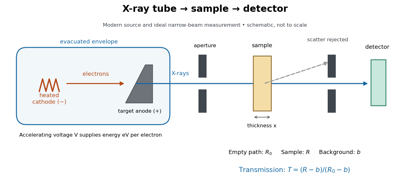
In bremsstrahlung, an electron changes velocity in the target's electric fields, emitting a photon while losing kinetic energy. Different encounters allow a continuous range of transferred energies. This is distinct from the discrete electronic transitions producing Characteristic X-rays.
Changing the accelerating voltage changes the available kinetic energy per electron and the X-ray tube cutoff. Changing the number of arriving electrons changes the number of opportunities for photon emission. These are distinct controls: a larger electric current does not by itself give each electron more energy. For an original idealized budget, and tube electric current give electrical power and arrival rate , where is the elementary charge. This is input power, not emitted X-ray power; obtaining the latter requires a conversion efficiency.
For an electron starting with negligible kinetic energy and accelerated through a constant positive electric potential difference , electrical work supplies . In the ideal single-electron bremsstrahlung model, conservation of energy bounds any one emitted photon:The endpoint corresponds to essentially all available kinetic energy going into one photon. It is a limiting bound, not a claim that every electron produces an endpoint photon. Neglect target recoil, initial kinetic energy, and losses before the emitting interaction. If the accelerating voltage varies, its largest value sets the corresponding ideal upper endpoint; a mean voltage does not substitute for that value.
For a calculated constant- example, gives and . Doubling halves . Producing a photon requires at least in this model. A continuous frequency spectrum spans lower photon energies; the cutoff calculation predicts neither its shape nor the efficiency of photon emission.
A Characteristic X-ray comes from an electronic transition filling an inner electron shell vacancy. The emitted photon carries the difference between atomic energies. Vacancy creation by direct electron impact requires kinetic energy above the shell's binding energy, exceeding the line energy. Higher tube voltage need not move the spectral line.[ref]
Chapter 5: X-Ray Production (teaching slides) by K. P. Maher. Diagnostic Radiology Physics: A Handbook for Teachers and Students; IAEA Chapter 5, §§5.2.2–5.2.3: shell vacancy, binding-energy threshold and characteristic radiation
An original stipulated shell model illustrates the distinction without using measured atomic data. Let positive binding energies be and , ignoring relaxation corrections. Filling a K-shell vacancy from the L shell releasesAn tube can energetically emit a bremsstrahlung photon, yet cannot directly remove this K-shell electron. A tube can create that vacancy by electron impact; if radiative filling occurs, the line is still , not . This argument concerns direct electron impact and an initially unexcited target; it does not describe every possible excitation route.
X-ray emission spectroscopy studies the frequency spectrum of emitted X-rays. The spectral line positions identify electronic energy differences; their strengths also depend on excitation, photon absorption inside the sample, geometry and detector response. An X-ray tube may excite a sample with electrons, while X-ray fluorescence uses incident photons. The distinction matters when choosing what the experiment measures: identifying a chemical element from a line position is different from determining its abundance from a line strength.
Charles Glover Barkla's 1911 paper describes irradiating a target with an X-ray tube and observing secondary X-rays using an electroscope. For soft Characteristic X-rays from tin, he used a soft primary beam and placed the electroscope close to the target to limit loss in air. Successive aluminium absorbers changed the gas-ionization signal. Thick absorbers suppressed the soft component; a carbon radiator supplied a comparison for the surviving scattered component. Subtracting this estimated contribution left approximately equal fractional losses through successive sheets, evidence for a nearly homogeneous component. Changing primary-beam hardness could suppress excitation of the more penetrating characteristic component.[ref]
The Spectra of the Fluorescent Röntgen Radiations by Charles Glover Barkla. Barkla, The spectra of the fluorescent Röntgen radiations (1911), p. 396: soft tube, nearby electroscope, aluminium sheets, carbon comparison and subtraction
An electroscope reads loss of stored electric charge; ionization in its detecting gas enables discharge. An ionization chamber with an electrometer instead measures the collected electric charge or electric current. These are integrating readouts: neither directly assigns an energy to each arriving photon. The diagram separates these functions without claiming a surviving apparatus drawing.
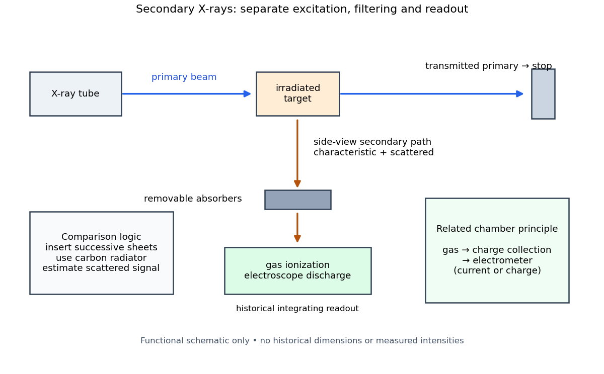
The K and L components were distinguished by their penetrating power and dependence on the emitting chemical element. Barkla's Nobel lecture, delivered on 3 June 1920 for the 1917 prize, explains that absorber-defined K radiation had seemed homogeneous, whereas later diffraction experiments resolved neighbouring spectral lines in both K and L groups. Absorber tests therefore distinguished groups without resolving every line.[ref]
Characteristic Röntgen Radiation by Charles Glover Barkla. Nobel Lectures, Physics 1901–1921; Barkla, Characteristic Röntgen radiation, printed pp. 392 and 395, PDF pp. 132 and 135: lecture date and limitations of absorption analysis
Henry Gwyn Jeffreys Moseley subsequently related the frequencies of corresponding spectral lines to atomic number. The approximate relation , with series-dependent constants , is Moseley's law; its discovery should be distinguished from Barkla's identification of characteristic secondary radiation.[ref]
Moseley and X Rays by University of Oxford Department of Physics. University of Oxford Department of Physics, Moseley and X rays: Moseley's graph and the story of Moseley and X-rays
A continuous incident frequency spectrum can contribute a continuous scattered background alongside discrete Characteristic X-rays. Here “scattered” identifies a production process, not a universal spectral shape: scattering of a narrow incident line need not make a continuum. In particular, the characteristic component is photon emission after vacancy creation, rather than simply the primary beam redirected. Source hardness, target substitution and absorber thickness probe different parts of that distinction. A surviving signal alone establishes neither an additional electron shell nor a fully resolved spectral line.
Precision X-ray emission spectroscopy turns closely spaced spectral lines into quantitative constraints on atomic energy levels. Bragg's law makes a crystal an angular ruler for wavelength: resolving nearby directions can reveal components hidden inside an apparently single line. Accurate line positions and the ability to separate two lines are related, but distinct, experimental achievements.
Karl Manne Georg Siegbahn received the 1924 Nobel Prize in Physics; his lecture was delivered on 11 December 1925.[ref]
The X-ray Spectra and the Structure of the Atoms by Karl Manne Georg Siegbahn. Nobel Lectures, Physics 1922–1941; The X-ray Spectra and the Structure of the Atoms, heading, printed p. 81
His son Kai Siegbahn received the 1981 Nobel Prize in Physics for electron spectroscopy.[ref]
Facts on the Nobel Prize in Physics by Nobel Prize Outreach. Family Nobel Prize laureates in physics, Father and son: Manne and Kai Siegbahn
The Barkla characteristic X-ray experiment distinguished element-dependent K and L groups through absorption and excitation. Moseley's law related corresponding line frequencies across chemical elements to atomic number. Measuring the components within those groups asks a further question: which distinct atomic energy differences produce the neighbouring spectral lines?
Siegbahn's lecture organizes measured spectral lines into energy levels and resolved double levels.[ref]
The X-ray Spectra and the Structure of the Atoms by Karl Manne Georg Siegbahn. Nobel Lectures, Physics 1922–1941; Printed pp. 84–86, Figs. 1–2
The payoff is a map of atomic energy differences as well as an element's position in the periodic table.A crystal X-ray spectrometer selects a narrow wavelength interval by diffraction at known interplanar spacing and Bragg angle . For fixed diffraction order , a known lets an angular measurement determine . This reverses the crystallography problem of finding from a known wavelength.
Siegbahn's laboratory developed X-ray tubes and evacuated spectrographs for longer wavelengths. Rotating the crystal selected reflections; photographic plates recorded positions. Opposite-side exposures measured angles on both sides of the direct beam. Later tube instruments mounted a beam-defining slit opposite the plate holder. A separate double instrument compared two reflected beams with two ionization chambers. These were different instruments, not one universal assembly.[ref]
Manne Siegbahn, His Research by Hugo Atterling. Hugo Atterling, Manne Siegbahn: Development of precision spectroscopy; Work at Uppsala 1923–1927
The Nobel biography describes constant-temperature spectrographs and a precision angular scale read by diametrically opposed microscopes.[ref]
Manne Siegbahn - Biographical. Nobel Lectures, Physics 1922–1941; Biographical, paragraph beginning As a measure of the high precision; inspected collected volume pp. 90–91
Temperature control matters because thermal expansion changes ; an accurately read angle cannot compensate for an unknown interplanar spacing.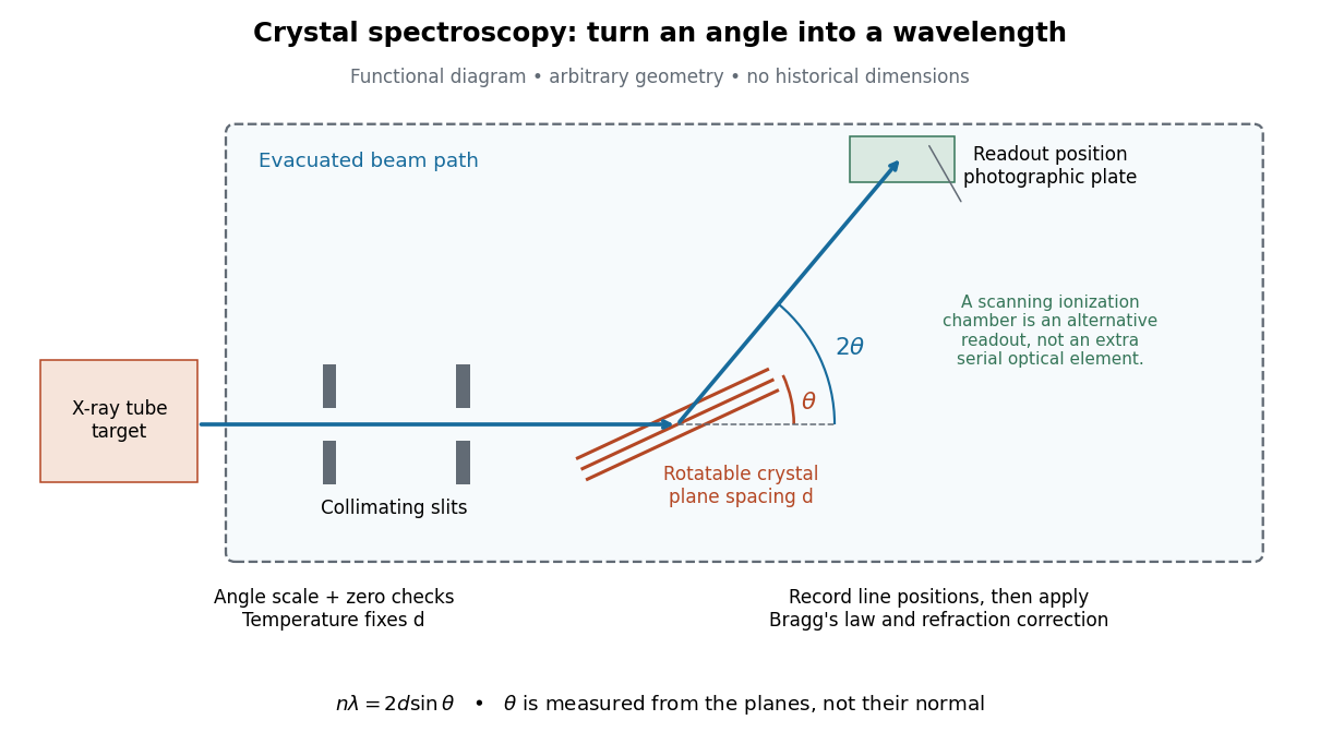
The schematic separates preparation, selection and readout. An X-ray tube target supplies Characteristic X-rays with a possible bremsstrahlung background. A collimator limits incident directions; evacuation reduces air X-ray attenuation. Rotating the crystal brings different wavelengths into reflection. A photographic plate stores line positions over an exposure, whereas an ionization chamber can measure collected electric charge at successive angles. Neither readout alone establishes absolute wavelength: an angular zero, angular-scale calibration, diffraction order, and any required refraction correction enter the inference. Narrower slits reduce accepted angular spread but also reduce signal; a weak line can become harder to locate despite a narrower instrumental response.
A control reported in Siegbahn's lecture photographed a line system with copper-sulphate and calcium-sulphate crystals. Irregular relative shifts around copper's characteristic frequency supported anomalous dispersion; the arrangement excluded differing absorption across that frequency as the explanation.[ref]
The X-ray Spectra and the Structure of the Atoms by Karl Manne Georg Siegbahn. Nobel Lectures, Physics 1922–1941; Printed pp. 88–89, final experiment
A finer angular scale alone cannot remove this physical refraction correction.Differentiate Bragg's law at fixed correctly assigned diffraction order:Divide the second equality by the first. For small signed changes,The Bragg angle error must be in radians. An error quoted for detector deflection must first be halved. The expression is a first-order Taylor expansion; an unknown diffraction order is a discrete assignment error, not an infinitesimal perturbation.
For error bounds, add magnitudes. For independent zero-mean random errors with standard deviations , variance addition instead givesCorrelated errors require a covariance term. A shared calibration bias does not become independent merely because many line positions are measured.
With a chosen angular error arcseconds, , the angular contribution is at and at . Larger Bragg angles reduce this contribution because decreases. For a nearby spectral doublet, the inverse relation is : a fixed fractional separation spreads farther apart angularly at large Bragg angle.
This does not permit unlimited improvement. The geometry requires ; a desired wavelength might not have an accessible large-angle reflection with the chosen crystal. Higher diffraction orders can reach larger Bragg angles but their strengths depend on the crystal lattice structure factor. Finite crystal response, slit widths and source size remain relevant. An error in , including uncorrected thermal expansion, remains even when the angular term is small. Very near , the leading angular derivative vanishes and the second-order Taylor expansion matters.
For two lines measured with the same interplanar spacing at the same temperature, division of Bragg's law givesThe common cancels. Consequently a precise wavelength ratio can coexist with an uncertain conversion to SI length. In contrast, angular calibration errors generally survive: a shared small zero offset changes the inferred ratio fractionally by approximately . Nearby lines partially cancel this effect, but widely separated angles need not. Different crystals, temperatures or refraction corrections also prevent unqualified cancellation.
The historical X unit was a practical X-ray wavelength unit, approximately . Its scale used an assigned calcite spacing; relative wavelength measurements could be more precise than absolute determinations. Variation between crystal specimens led to calibration using reference spectral lines. An X unit value therefore cannot simply be read as an exact multiple of .[ref]
Nomenclature System for X-ray Spectroscopy prepared by R. Jenkins and others. IUPAC, Nomenclature system for X-ray spectroscopy, §5.1 Units, printed p. 745
An angular-scale check determines how an indicated rotation corresponds to an angle. A reference line transfers a wavelength scale. An absolute determination ties that scale to an independently established length standard. These are different calibration tasks. Repeating measurements can reduce random scatter without correcting the common scale: if every inferred is too large by a chosen , all inferred absolute wavelengths are too large by , while ratios using that same are unchanged.
A spectral doublet comprises two neighbouring spectral lines. Resolving it requires information about the line response, relative strengths and noise, not only precision in reading an angle. Choose two equal angular responses shaped as Gaussian functions with common standard deviation and separation . If is angular displacement from their midpoint, their summed signal isThese are assumed response shapes, not a measured Siegbahn frequency spectrum. By symmetry , andThe midpoint changes from a maximum to a minimum at . For this particular equal-width, equal-height model, two distinct maxima occur when . Each isolated Gaussian function has full width at half maximum ; the two-maxima threshold is therefore about times that width.
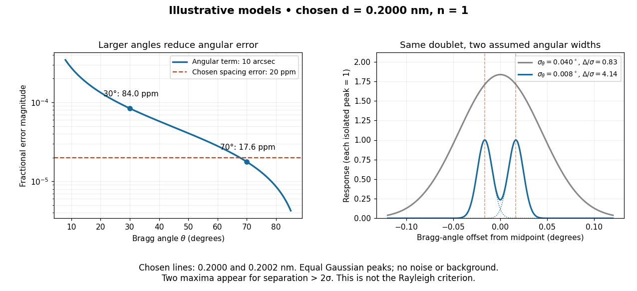
In this chosen model, the two Bragg angles are and . Their separation is times for , giving one maximum, and times for , giving two. Sharpening the response can reveal the doublet without changing either emitted wavelength.
The Rayleigh criterion uses a first-zero convention for specified diffraction patterns. A Gaussian function has no finite zero, so its two-maxima threshold is not the Rayleigh criterion. Neither convention is a universal inference limit: known response shapes and adequate signal-to-noise ratio can support estimating a separation before two visible maxima appear. Unequal strengths, background, finite sampling and uncertainty in the response can make that inference much harder. Measurement resolution, the precision of an isolated line's centre and absolute wavelength accuracy should therefore be reported separately.
For a fixed homogeneous absorber in a narrow-beam geometry, define the X-ray spectral attenuation operator on L1 space over a bounded positive energy interval. A physical input is an integrable function giving incident photon rate density. Let its linear attenuation coefficient be a measurable function, with . The transmitted uncollided density isHere is a fixed bounded detector response described by a measurable function; background has been subtracted. This is a positive linear operator on L1 space. Since , it cannot increase the integrated absolute incident rate. Multiplication of exponentials proves for successive layers of the same material. Ignore secondary radiation entering the detector, saturation and changes to the source. Discrete spectral lines use the finite-sum version below instead of an ordinary rate density.
For a chosen filter, stipulate , and input line rates in a common arbitrary rate unit. Assume equal calibrated detector weight for both lines. At ,The selected line's fraction rises from to , but its absolute rate falls by about . Filtering improves purity at the cost of signal. It multiplies existing components and cannot create a new emitted spectral line.
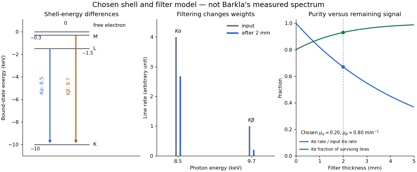
With just one integrated reading, , the two unknown line rates are underdetermined. If the source is unchanged between an empty-path reading and a filtered reading, the ideal inverse problem becomesThe determinant is nonzero, so these two ideal readings determine the two stipulated line rates uniquely. Identical coefficients would give zero determinant and destroy that separation. This small linear algebra example explains why absorber contrast supplies information, while also showing its limit: unknown scattered components or unknown detector weights add unknowns that two readings cannot determine.
X-ray fluorescence is Characteristic X-ray emission following excitation by incident photons. In a simple initially unexcited chemical atom, photoionization can eject an inner electron if the incident photon supplies its binding energy. An outer electron can then fill the vacancy, releasing an emitted photon with the difference of shell binding energies. Nonradiative relaxation competes with this route, so one absorbed incident photon need not yield one escaping characteristic photon.
Choose a separate stipulated electron shell model with values , and , all in . Ignore subshell splitting, recoil and changes of binding energy during relaxation. The possible shell differences areThese labels denote simplified shell groups, not resolved subshell electronic transitions. With , their calculated wavelengths are respectively , and . An incident photon exceeds both K-line energies but cannot directly create the K vacancy in this initially unexcited model. A photon can, leaving approximately of photoelectron kinetic energy. This comparison fixes neither the excitation probability nor the radiative branching probability.
For a narrow beam of monoenergetic photons crossing homogeneous material of thickness , the uncollided wave intensity obeys . Here is the linear attenuation coefficient, counting removal from the incident beam by photon absorption and scattering of light. It depends on photon energy and material; it is not universally independent of energy.[ref]
2. The Mass Attenuation Coefficient. Tables of X-Ray Mass Attenuation Coefficients and Mass Energy-Absorption Coefficients by John H. Hubbell and Stephen M. Seltzer; NIST, X-Ray Mass Attenuation Coefficients, §2, Eq. (1), narrow monoenergetic beam and interaction contributions
An original derivation makes the model explicit. If each thin layer removes fraction of the surviving beam, with the same throughout, thenThus equal added thicknesses multiply transmission by the same factor. The ordinary differential equation describes uncollided beam survival. To test it with a detector, keep source output, distance, selected photon energy band and detector response fixed. Use a collimator and suitable detector acceptance to exclude scattering of light into the detector. Subtract background, measure an empty-path reference, and keep the detector in its linear operating range. A changing source distance adds geometric dilution and is not an attenuation measurement at fixed geometry.
For a stipulated example, take and . Transmission is . If the empty-path detector rate is , including background , the model predicts sample rate . Recover transmission as ; the raw ratio is biased. These chosen values are a calculation, not measurements of a particular material or a historical apparatus.
When X-ray transmission is exponential, and when spectral mixing bends it
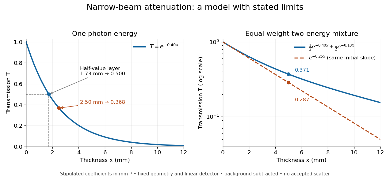
. Original calculated examples, with stipulated linear attenuation coefficients in inverse millimetres. The left panel uses one photon energy and marks and the half-value layer. The right panel compares an equal-weight mixture of two photon energies with the exponential having the same initial slope. A logarithmic vertical axis turns a single exponential into a straight line. Neither curve is fitted to measured material data. Details.The linear attenuation coefficient is the infinitesimal probability of removal from the uncollided beam per unit path length. Its units are inverse length. In the homogeneous monoenergetic model, ; is the thickness leaving fraction uncollided. The mass attenuation coefficient is for material mass density . Removing a photon by scattering of light does not imply deposition of all its energy at that point; attenuation and energy absorption are different quantities.[ref]
2. The Mass Attenuation Coefficient. Tables of X-Ray Mass Attenuation Coefficients and Mass Energy-Absorption Coefficients by John H. Hubbell and Stephen M. Seltzer; NIST §2, mass thickness, Eq. (1), and total interaction cross section; distinction from the mass energy-absorption coefficient
A coefficient describing the locally absorbed fraction of an incident photon energy flow per path length, under a stated averaging convention. It is distinct from the total linear attenuation coefficient, which counts removal from an uncollided beam. Dividing by mass density gives an energy-absorption coefficient per mass.
The uncollided component decays exponentially when its removal probability per unit path length is constant. Scattered contributions require a separate transport treatment or a specified radiation buildup factor.
The linear attenuation coefficient divided by the material mass density.
An energy-weighted interaction coefficient for photons, accounting for the fraction transferred to charged particles after radiative losses. It differs from the removal-probability mass attenuation coefficient. With charged-particle equilibrium, its product with photon energy fluence gives the absorbed dose.
The half-value layer is the thickness reducing the specified transmitted signal by one half. For constant monoenergetic linear attenuation coefficient , solving gives . The stipulated gives ; two such layers transmit one quarter. A broad frequency spectrum need not retain the same half-value layer after filtering.
An original two-energy model demonstrates the failure of a single constant linear attenuation coefficient for a mixed beam. Suppose the two components contribute equally to the empty-path detector signal and have stipulated and . With fixed linear detector response and no accepted scattering of light,The initial slope corresponds to , but at , , rather than . The more strongly attenuated component disappears faster. If that component has lower photon energy, the surviving beam has a higher mean energy: beam hardening. The formula is explicitly a two-component example, not a universal rule that attenuation decreases monotonically with photon energy. Detector weighting also matters when interpreting a broadband transmission signal.
An absorption edge is an abrupt change in photon absorption as incident photon energy crosses an electronic excitation threshold. For inner-shell photoionization, a new vacancy-production channel opens near the shell's binding energy. This threshold concerns incident energy; a Characteristic X-ray concerns a subsequent difference of atomic energies. They are different observations. Barkla's lecture explicitly treats characteristic emission as requiring a critical excitation condition, while discussing characteristic radiation separately from scattering.[ref]
Characteristic Röntgen Radiation by Charles Glover Barkla. Nobel Lectures, Physics 1901–1921; Barkla, Characteristic Röntgen radiation, printed p. 395, PDF p. 135: shorter-wavelength excitation and critical condition
In the stipulated X-ray fluorescence model, the K threshold is , whereas the K lines are and . An absorber made of a different material could have its own absorption edge between those line energies, preferentially removing the upper line. Actual near-edge structure and attenuation values require material data; the following deliberately chosen coefficients are not such data.