A covariance matrix describes second moments, but does not specify a complete probability distribution. A bounded model can realize a prescribed covariance matrix exactly while keeping every possible error finite. This is useful for checking a nonlinear measurement model without accidentally generating physically impossible inputs; it is a constructed model, not evidence that an actual instrument has that distribution.
For two errors with desired standard deviations and correlation coefficient , let be independent random variables with the Rademacher distribution: each takes and with probability . SetBoth expected values vanish. Since and , direct expansion givesThere are at most four distinct states, each obtained from an equally likely sign pair. Also and . At the second sign has no effect, leaving only two distinct states. If either standard deviation is zero, the corresponding error is zero and its correlation coefficient is undefined; the covariance construction still makes sense.
More generally, a finite-support realization of a covariance matrix exists for every real symmetric positive semidefinite matrix . By the spectral theorem, write using its positive eigenvalues and corresponding orthonormal eigenvectors, and put . Let have independent Rademacher distribution coordinates. The random vector then satisfiesThe identity matrix appears because the signs have unit variance and zero pairwise covariance. There are at most distinct states, with component bounds by the Cauchy-Schwarz inequality. When , take . Thus singular covariance matrices are allowed; a nonsingular Cholesky decomposition is not required.
This full sign model also makes robust linear constraints for bounded covariance models exact. To require for every sign state, choose each sign to minimize its contribution. The result is the necessary and sufficient conditionwhere is the L1 norm. This is a small robust optimization calculation. A physical domain must be checked in the chosen units; clipping inadmissible samples afterwards generally changes both the probability distribution and its covariance matrix.
For example, in correlated threshold and amplitude errors in RC timing, take nominal amplitude , threshold , , and . Use and . Every state has , while the minimum amplitude-minus-threshold isAll four states therefore remain within the RC threshold-crossing time domain. Enumerating them supplies an exact check for this particular bounded error model; it does not establish the instrument's actual tail probabilities.
The nonuniqueness of bounded uncertainty laws with a fixed covariance is visible even in two dimensions. LetFor independent fair signs , both and have covariance matrix because is an orthogonal matrix. Yet the first coordinate of is always , whereas that of is with probability and each of with probability . Hence is respectively zero and one half, despite identical expected values and covariance matrices. A nonlinear risk calculation needs more than those moments.
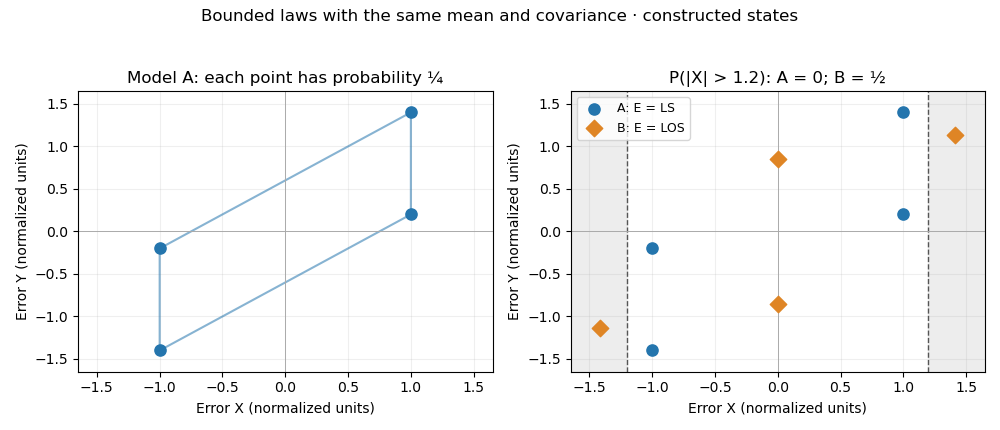
Two bounded four-state error models with identical covariance and different tail probabilities. All points are constructed, not measured data.
Details. 
Nonuniqueness of bounded uncertainty laws with a fixed covariance means that specifying finite bounds, expected values and a covariance matrix can still leave several different joint probability distributions. They agree on the variance of every linear combination of the errors, but can disagree on threshold probabilities and nonlinear outputs. A particular construction in bounded errors with prescribed correlation therefore requires a distributional assumption beyond its second moments.
Here is an original example with a common allowed box . In model A, and are independent fair signs: the four points each have probability . In model B, the four points each have probability . Both are bounded, have zero expected value, and satisfyFor model B, each squared coordinate is two at two of the four points and zero otherwise, proving its unit variance directly. Its zero covariance does not make the coordinates independent random variables: when is nonzero, must vanish. The common box is an allowed deterministic bound; its boundary need not be attained by every model.
The linear output has expected value zero and variance two under either model. Yet under model A it takes with probabilities , while model B gives only with equal probabilities. Consequently,Even a linear output's threshold risk is not fixed by its variance. For the nonlinear output , model A gives always and model B gives always. Thus the complete output law, and even a nonlinear output's expected value, can differ.
The law of propagation of uncertainty computes first-order output variance from sensitivity coefficients and input covariance; it does not identify all probabilities. NIST correspondingly requires distributional justification to assign a confidence level to an uncertainty interval.[ref]
Guidelines for Evaluating and Expressing the Uncertainty of NIST Measurement Results by Barry N. Taylor and Chris E. Kuyatt. Appendix A.3 and §§6.2–6.3
The finite counterexample above is an original exact calculation. For guaranteed linear limits, robust linear constraints for bounded covariance models must use the chosen support of a probability distribution, rather than treating a covariance matrix as a support description.Robust linear constraints for bounded covariance models require a linear inequality to hold for every error state admitted by the selected bounded model. A covariance matrix fixes second moments; the robust guarantee additionally depends on the support of a probability distribution or other specified uncertainty set. This distinction matters when a physical limit must never be crossed within the model.
Let as in finite-support realization of a covariance matrix, where all coordinates of are independent fair signs. Then . For nominal input , require for every sign state. Writing , direct minimization givesEach sign can independently oppose its coefficient, including when some coefficients vanish. Thus the exact necessary and sufficient condition is , using the L1 norm. The same extremum holds over the full box because a linear function attains an extreme at a vertex. This is a support function calculation in robust optimization; the general worst-case formulation and its dependence on the uncertainty set are illustrated in the primary optimization text.[ref]
Convex Optimization by Stephen Boyd and Lieven Vandenberghe. §4.4.2, printed p. 157, robust linear programming, equation (4.37); the text's illustrated uncertainty set is an ellipsoid
For an original two-input example in volts, let and , with independent fair signs . The covariance matrix is . To keep the actual first input at least as large as the second, let the nominal difference be . ThenA nominal difference of fails in the state , despite being positive nominally. A difference of leaves a guaranteed margin under this model. Using only the separate bounds , would demand , because that larger box admits joint states the sign model forbids.
The standard deviation of is instead . It is not the hard bound . A different bounded law with the same covariance matrix can change the hard bound, as nonuniqueness of bounded uncertainty laws with a fixed covariance explains. For several linear inequalities, apply the support calculation to each row. This verifies an assumed model's feasible states; it does not establish that the chosen support contains every error of an actual instrument.
Articles by others on the same topic
There are currently no matching articles.