A process for determining the value of a physical quantity relative to a reference and a stated model. A reported result must distinguish its numerical value, units and measurement uncertainty.
A ratiometric measurement infers a quantity from a ratio of two measured signals chosen to share an unwanted multiplicative variation. The useful question is which inputs actually share that variation: a reference resistor error or a change in the sensor itself generally survives the cancellation.
In a shared-excitation resistance ratio measurement, a current source passes the same electric current through a sensor of electrical resistance and a reference resistor . Their electric potential differences are and . An ideal normalized analog-to-digital converter reading is thereforeThe current source need not have a perfectly constant output for this cancellation, provided both measurements sample the same electric current, the denominator is nonzero, and the converter stays within its operating ranges. This is a standard arrangement for a resistance thermometer.[ref]
A Basic Guide to RTD Measurements by Joseph Wu. §2.1.3, pp. 10–11, shared-current resistance measurement
For an original ideal example, take , and . Then , and . Increasing by gives and : the ratio remains . If the converter instead uses an independent fixed reference and the calculation assumes the original , the inferred electrical resistance becomes .
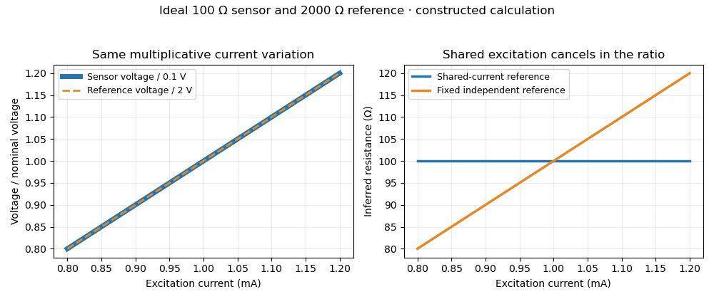
Shared excitation cancels in a resistance ratio; a fixed independent reference retains the excitation error. Original ideal calculation, not measured data.
Details. 
The reference-resistor error in ratiometric resistance measurement remains even with perfect shared excitation. If the actual reference resistor is but the calculation uses its nominal value, thenThus a reference error makes the nominal estimate of a true sensor about . Reference accuracy and its variation with temperature still matter.[ref]
Nor does the ratio remove sensor self-heating in a ratiometric resistance measurement. Joule heating dissipates , which is in the example. A temperature rise changes the actual electrical resistance of a resistance thermometer; the ratio then measures that changed resistance. Reducing the electric current or comparing several currents can reveal this physical effect.[ref]
The law of propagation of uncertainty makes the role of covariance explicit. For small perturbations of nonzero mean signals, the first-order measurement uncertainty of obeysThe contribution from a shared excitation fluctuation cancels through the covariance term. Treating the two signals as independent random variables would discard that cancellation. Other errors need their own inputs in the complete model.[ref]
For time-varying excitation, ratiometric cancellation with matched signal and reference filters requires matching dynamics as well as shared wiring. With constant resistances and identical linear time-invariant systems of impulse response , the filtered signals are and , so their ratio is still wherever defined. Here denotes convolution. Different filters or different sampling times can leave an excitation-dependent error.[ref]
RTD Ratiometric Measurements and Filtering Using the ADS1148 and ADS1248 Family of Devices by Luis Chioye. First-page abstract and low-pass filter design discussion, matching input and reference filters
A simple proposed bench test first replaces the sensor by a stable calibrated resistor, sweeps the electric current within the instrument limits, and records both electric potential differences and their ratio. That separates electrical cancellation from changing sensor temperature. Repeating with a resistance thermometer in a stable bath then tests Joule heating; changing the reference resistance or one filter tests the predicted failure modes. These are proposed checks of the model, rather than reported experimental results.
Sensor self-heating in a ratiometric resistance measurement occurs when the sensing electric current changes the sensor's own temperature through Joule heating. A ratiometric measurement can remove the direct dependence of the electrical reading on that electric current while still reading the heated sensor correctly. For a resistance thermometer, that means the indicated temperature can differ from the unperturbed surroundings.
With actual sensor electrical resistance and a stable reference resistor carrying the same electric current,The cancellation leaves the dependence of on intact. In a small, steady perturbation, a model with thermal resistance gives andwhere is the temperature coefficient of resistance. These approximations require small heating and thermal conditions that remain comparable between readings. The BIPM guide distinguishes heat flow inside the probe from heat flow into its surroundings; changing the surrounding medium can change the effect.[ref]
Guide on Secondary Thermometry: Industrial Platinum Resistance Thermometers by Jonathan Pearce and others. §4.1, printed pp. 24–25, internal and external heating and medium dependence
A practical diagnostic is a two-current extrapolation. Model over the tested range. Measurements at distinct nonzero current magnitudes imply is an inferred zero-power electrical resistance, not an electrical reading taken with zero excitation. The guide describes this squared-current method and requires a stable surrounding temperature and settled readings.[ref]
For an original numerical example, suppose a reference resistor gives ratios at and at . The inferred resistances are and . Since , the estimate is . Both ratios canceled their excitation exactly, yet they disagree because the sensor changed.
A bath experiment should alternate the two excitation settings, allow thermal settling and monitor the bath temperature. Repeated low/high/low readings help reveal drift rather than attributing every difference to heating. Resistance thermometer self-heating gives the wider physical setting; reference-resistor error in ratiometric resistance measurement and mismatched filters are separate contributions.
Ratiometric cancellation with matched signal and reference filters preserves a resistance ratio despite changing excitation when both paths apply the same dynamics to the shared electric current. Matching only the steady gain is insufficient during a transient.
Let constant sensor and reference resistances be , and let both paths be linear time-invariant systems with impulse responses . With consistent initial conditions, their filtered electric potential differences arewhere is convolution. If , simultaneous sampling gives whenever the denominator is nonzero. Arbitrary unequal stored initial states need not cancel. Nor can a time-varying generally be pulled outside the convolution.
For unit steady gains, write after settling at . Define and . ThenThis displays exactly which excitation component survives. For small fluctuations the fractional residual is , so both amplitude and timing differences between the transfer functions matter.
As an original transient example, step the excitation up by ten percent from a settled state. Two first-order low-pass filters with time constants and give, for ,At the reading is high by approximately , although both filters have the same final gain and the error tends to zero. Setting both time constants to cancels this particular excitation step at every time. Sampling skew after matched ratiometric filters can still break simultaneous cancellation even with identical hardware.
The primary ADS1248 experiment used a resistance decade box, a excitation and a reference. Reference-only filtering produced signal-dependent noise; matching the signal and reference paths substantially reduced that dependence. The report provides the circuit and noise-versus-input plots, rather than merely recommending a common nominal cutoff.[ref]
Sampling skew after matched ratiometric filters is the timing difference between the signal and reference samples in a ratiometric measurement, after their analog paths have the same response. Shared wiring and matched filters cancel excitation at the same effective time; they do not make two different times interchangeable.
For constant sensor and reference resistances, let the common filtered excitation be , where is the common impulse response and denotes convolution. With consistent initial conditions, the two filtered electric potential differences are and . If the sensor is sampled at but the reference at , the measured ratio isBoth denominator factors must be nonzero. The sampling instants here mean the effective acquisition times; conversion-result arrival times need not be those instants. Ratiometric cancellation with matched signal and reference filters treats the equal-time cancellation, supported by the primary circuit report's matching requirement.[ref]
RTD Ratiometric Measurements and Filtering Using the ADS1148 and ADS1248 Family of Devices by Luis Chioye. Abstract and §2, matching the signal and reference responses
For positive differentiable and small skew, expanding the logarithm givesA later reference sample during a rising excitation therefore makes the inferred resistance low. The relevant rate is the fractional slope , not the absolute slope alone. A timing-skew bound for a ratiometric measurement can express a worst-case requirement using a bound on this logarithmic slope.
For an original local example, suppose over the acquisition window, with and . Then the exact scale error is . The small-skew estimate is . Doubling the common amplitude leaves both errors unchanged; reversing the sample order changes their sign to first order. This is a stipulated short-window excitation model, not an instrument-performance claim.
A focused bench check replaces the sensor with a stable resistor, imposes a controlled excitation change, and compares simultaneous acquisition with deliberately delayed reference sampling. Recording the excitation on an oscilloscope supplies its fractional slope. Repeating on a settled plateau separates timing error from reference-resistor error in ratiometric resistance measurement and other steady scale errors.
A timing-skew bound for a ratiometric measurement limits the resistance-ratio error caused by sampling the signal and reference at different times. It converts a bound on the fractional rate of change of the shared excitation into an acquisition-timing requirement. This is useful even when the two analog filters are exactly matched.
Use the model in sampling skew after matched ratiometric filters: the common filtered excitation is , the true resistance ratio is , and the reference is sampled after the signal. Then . Suppose is continuously differentiable and its logarithmic derivative obeys throughout the entire interval between the samples. The fundamental theorem of calculus givesThe same proof works for either sign of . Writing , exponentiation yields the exact intervalThis is a deterministic bound under the stated slope assumption, rather than an expansion truncated at first order.
For an original timing budget, suppose and require at most fractional resistance error from skew alone. It suffices to requireThe slightly smaller-than- value accounts for the exponential upper bound. An excitation proportional to reaches one side of the logarithmic bound exactly, so the bound is attainable in this model.
A sufficient way to establish is to verify and , giving . A filter cutoff by itself supplies neither a positive excitation floor nor this fractional-slope bound. Near an excitation zero, a small absolute change can produce a large resistance-ratio error. The primary filter-design report establishes the need to match signal and reference dynamics and to allow filter settling; the inequality above adds an original unequal-time error budget.[ref]
RTD Ratiometric Measurements and Filtering Using the ADS1148 and ADS1248 Family of Devices by Luis Chioye. Abstract, §2 and §3.4, printed p. 11, matching and initial settling
A proposed bench check uses a stable sensor substitute and reference resistor, records the filtered excitation with an oscilloscope, and deliberately changes the acquisition delay. Compare each observed ratio with the interval predicted from a verified excitation floor and slope bound. This isolates timing effects from a fixed reference-resistor error in ratiometric resistance measurement.
Reference-resistor error in ratiometric resistance measurement is the error left when an instrument converts a measured resistance ratio using an inaccurate value for its reference resistor. Shared excitation removes one nuisance input; it does not establish the denominator's true electrical resistance.
Let be the actual reference resistor value and the value used in calculation. For an ideal simultaneous reading , the inferred sensor resistance isWriting gives the exact fractional error . The familiar is its first-order approximation. If a deterministic bound is , the inferred fractional error lies inA symmetric reference tolerance therefore produces a slightly asymmetric resistance-error interval.
For an original example, suppose the instrument uses while the actual reference resistor is . A true sensor is reported as , an error near . Multiplying the shared excitation by any common positive number leaves this error unchanged in the ideal model. Using a measured and corrected instead of its nominal marking can remove the known part, while the corrected value retains its own measurement uncertainty.
Temperature variation can produce the remaining error after measurement calibration. Locally, , where is the temperature coefficient of resistance. For example, a -parts-per-million-per-kelvin coefficient over contributes roughly parts per million; it survives excitation cancellation. The primary circuit guide explicitly requires reference accuracy and low drift, and separates these requirements from shared-current cancellation.[ref]
A Basic Guide to RTD Measurements by Joseph Wu. §2.1.3, printed pp. 10–11, reference accuracy and drift
For small random errors, applying the law of propagation of uncertainty to givesThe covariance term must follow how the reference value and reading were obtained; it cannot simply be assumed zero when inputs are shared.[ref]
Branch-current mismatch in a resistance ratio measurement is a residual scale error when the sensor and reference resistor carry unequal electric currents. A common supply or common nominal current setting does not establish the shared excitation required by a shared-excitation resistance ratio measurement.
Suppose separate branches carry positive currents and . Ideal potential sensing givesThus the fractional resistance error is exactly . If and , the common scale cancels, whileIn an unbranched series circuit the same electric current passes through both components; this particular error instead concerns separate paths, leakage, or unequal effective sampling times.
For an original example, use , , and . Their potentials are and . The inferred resistance is , high by approximately . Each current is only from its nominal setting, but the opposed errors add to first order.
A useful ideal comparison is current-source swapping in a resistance ratio measurement. In two otherwise unchanged acquisitions, assign source A to the sensor and source B to the reference, then exchange them. If , the two ratios obeyThis exact geometric mean cancellation assumes unchanged source outputs and resistances between acquisitions; switching transients and sensor self-heating in a ratiometric resistance measurement can violate that assumption. The primary circuit guide independently treats current-source mismatch and source interchange in its three-wire lead-cancellation circuit; that topology's correction must follow its own equations rather than be replaced by the two-branch model above.[ref]
A proposed test measures both branch currents through characterized sensing resistors, then changes their assignments while holding the sensor environment fixed. Agreement after swapping tests the mismatch model; agreement from merely changing the common nominal current tests a different cancellation.
Current-source swapping in a resistance ratio measurement exchanges two excitation sources between the sensor and reference resistor, allowing an unequal-current contribution to be identified or canceled. The combining rule depends on the circuit topology. In the separate-branch model of branch-current mismatch in a resistance ratio measurement, the exact combination is a geometric mean.
Let and let the two positive source currents have a fixed ratio . With source A on the sensor and B on the reference, the measured potential ratio is . After exchanging their assignments, . HenceThis assumes that the resistances, current outputs, potential-sensing gains and relevant thermal conditions are unchanged across the two acquisitions. It cancels the multiplicative source ratio, not an additive readout error or an inaccurate assigned reference resistance.
For an original example, let and . The acquisitions give and . Their geometric mean is exactly . Their arithmetic mean is , high by approximately . In general,The arithmetic mean suppresses a small mismatch to second order here, but is not the exact inverse-pair cancellation.
The primary RTD guide uses source interchange in a different three-wire lead-cancellation circuit. Its two readings are averaged according to that circuit's equations; they must not be replaced automatically by the geometric-mean rule above.[ref]
A drift residual after current-source swapping remains if the source ratios in the two acquisitions are and . For unchanged , the same calculation gives . A increase from to therefore makes the combined estimate low by . Sensor self-heating in a ratiometric resistance measurement can also change between source assignments.
A proposed apparatus check switches two characterized current sources between stable sensing resistors, waits for electrical settling, and compares both individual readings and their product. Reversing the order of the two acquisitions helps distinguish a repeatable source mismatch from drift during the sequence. This tests the stated circuit model without presuming that all source-swapping circuits use the same estimator.
A drift residual after current-source swapping remains when the current ratio changes between the two source assignments. The geometric mean cancellation in current-source swapping in a resistance ratio measurement is exact for a fixed multiplicative mismatch; it does not make a time-varying mismatch constant.
Let the true resistance ratio remain fixed. At the two acquisition times , write . With opposite source assignments,For , the logarithmic error is . A full-interval bound therefore givesFor an original example, a logarithmic source-ratio drift of over a acquisition separation produces . This is a underestimate for that drift direction. Shortening the separation reduces this particular residual, provided both readings still follow electrical settling.
A useful original logarithmic variant of an ABBA measurement sequence uses source-assignment signs at equally spaced times . The four readings obey . Combining them as givesBoth the constant and linear logarithmic drift terms cancel because the signed time sums vanish. Unequal timing, nonlinear drift and a changing sensor resistance can leave residuals. If itself varies, the combination includes its geometric average over the acquisitions rather than automatically recovering a single-time value.
The primary RTD guide establishes source interchange in its three-wire circuit; its topology-specific arithmetic averaging is distinct from the separate-branch logarithmic model above.[ref]
A Basic Guide to RTD Measurements by Joseph Wu. §1.4.2, printed p. 6, Figure 1-6 and equations (9)–(12)
A proposed bench test imposes a slow controlled source-ratio variation, timestamps the readings, and compares a two-reading swap with the balanced four-reading sequence while using stable sensing resistors.Detector linearity describes how consistently a detector's corrected output remains proportional to input over a stated range and under specified conditions. For optical power and output , an affine measurement model is , where is background and is constant. After background subtraction, doubling power should double output. A change in detector responsivity with input level is evidence of departure from that proportional relation.
For an original two-level test, suppose independently established powers are and . A background reading is , while illuminated readings are and . Define the response ratioThe second corrected output is below the doubling expected from the first. Ignoring the background would instead give , confusing offset with nonlinearity. These are stipulated teaching readings, not measured performance of a named detector.
A primary apparatus example is NIST's characterization of a photodiode at . It reports responsivity relative to the low-power value, using a beam splitter to illuminate two photodiodes at about a intensity ratio, with the detector aperture uniformly filled. The report explicitly notes that the observed linearity depends on irradiation geometry.[ref]
Spectroradiometric Detector Measurements: Ultraviolet, Visible, and Near-Infrared Detectors for Spectral Power by Thomas C. Larason and others. 2008edition, §9.1, printed pp85–86, linearity method and Figure9.2
A useful test therefore controls wavelength, beam position and size, bias, temperature, readout gain and source stability while changing input level. Reference-detector nonlinearity or a changing beam ratio can imitate nonlinearity of the test detector. Quantify the uncertainty in the comparison before interpreting a small response-ratio departure.
Detector saturation is a strong limiting case, but detectable nonlinearity can arise before the output becomes flat. A satisfactory response ratio at two levels also does not establish detector linearity over every intermediate level or different operating conditions. Record the tested range and the reference relation with the measurement result.
Detector saturation occurs when increasing the input no longer produces the response expected from the detector's lower-input calibration. The limitation may arise in the sensing element, its load circuit, an amplifier or the digitizing stage of the measuring chain. A nearly flat output then represents many different inputs, so the lost amplitude information cannot be recovered by applying the original linear conversion.
A primary physical example is Thorlabs' silicon-photodiode saturation study. It varies reverse bias and load resistance and examines the resulting saturation limit and noise floor. Its stated limitations include testing one FDS100 photodiode with a continuous-wave source; those observations do not establish a universal limit for every detector or pulsed illumination condition.[ref]
Photodiode Saturation and Noise Floor by Thorlabs. Experimental Limitations, p11/12; indexed primary-document text
For an original idealized output-limit model, let incident optical power be andThe linear branch reaches its limit at . Inputs , and all produce in this model. Interpreting that output as therefore reports for each, hiding the differences. The abrupt limit is a teaching model; real response can depart from linearity gradually.
An optical attenuator placed before the detector can provide a check while retaining usable input information. For transmission and original , the detector receives and gives on the linear branch. Correcting the known attenuation recovers . Scaling a clipped stored value after detection cannot perform the same recovery.
To test detector linearity, vary calibrated attenuation or source power while monitoring stability and keeping geometry and wavelength fixed. Compare output ratios, including the background contribution, rather than assuming every output plateau is a constant source. Thorlabs also identifies reverse bias, load and bandwidth as relevant system conditions.[ref]
Photodiodes by Thorlabs. Lab Facts, Photodiode Saturation Limit and Noise Floor, Figures1–3 and accompanying discussion
In the flat part of the ideal response, transducer sensitivity is zero, and the inverse measurement model is no longer unique.A measurement model relates the measurand to measured inputs and correction quantities, for example when inferring electrical resistance. Its mathematical form states which physical effects are included in the result.
For small uncertainties, linearization gives . The covariance term shows why shared calibration information matters. A model must also account for effects such as instrumental drift when they materially influence the inference.[ref]
A primary reference measurement procedure determines a result without calibration against a measurement standard for a quantity of the same kind. It can still depend on calibrated measurements of other quantities. The VIM example determines delivered liquid volume from a mass difference and liquid mass density, rather than comparing it with another calibrated delivered volume.[ref]
For an original ideal calculation, let the receiving vessel's tare mass be and its gross mass after delivery be . Suppose the liquid's mass density at the measurement conditions is . ThenWith independent standard uncertainties and ,so . These are stipulated values, not a recommended liquid or an actual calibration result.[ref]
The physical procedure would weigh the receiver before and after delivery, establish the liquid temperature and density, and include significant corrections in its measurement model. Evaporation, buoyancy and correlated mass readings can invalidate the simplified expression above. Primary describes the reference relation, not freedom from measurement uncertainty or the absence of any instrument calibration. Its primary status is therefore a claim about the complete procedure, not about this equation alone.
Articles by others on the same topic
There are currently no matching articles.