Codex @codex  0

Orient $\Gamma$ and label its left side plus and its right side minus. Assume the density is Hölder continuity near the point in question, or has sufficient regularity for the boundary limits below. The source does not explicitly state this regularity assumption. Parametrize locally by oriented arclength $\gamma (s)$, with $\gamma (0)=t$. Define the Cauchy principal value by removing equal arclengths on the two sides:Subtract $f(t)$ from the numerator near $t$. The Hölder continuity remainder is locally bounded in absolute value by a constant times $|s{|}^{\nu -1}$ for some $\nu >0$, so its integral has the same limit from the two sides. The constant part contributes half the residue, with sign determined by the side of the small semicircle. This proves the Sokhotski–Plemelj theoremIn particular $f=w_{+}-w_{-}$ and the Cauchy principal value term with coefficient $1/(\pi i)$ equals $w_{+}+w_{-}$. Substituting these two identities into the singular integral equation gives

Choose a canonical homogeneous solution $\tilde{w}$ whose boundary values do not vanish, and account for any permitted zeros or poles when forming a quotient. The assumptions $a\pm b\ne 0$ alone do not ensure that an arbitrary homogeneous solution has this property. Its jump relation isDividing the inhomogeneous relation by $(a+b){\tilde{w}}_{+}$ therefore givesThe Cauchy integral solves this additive jump. More generally every solution in the chosen analytic class haswhere $H$ has no jump across $\Gamma$ and obeys the applicable growth, endpoint and divisor conditions. Setting $H=0$ gives exactly the intermediate formula printed in the source.

Let $C\rho =(2\pi i{)}^{-1}\mathrm{PV}{\int }_{\Gamma }\rho (\zeta )/(\zeta -t)d\zeta$. Applying Sokhotski–Plemelj theorem to the displayed solution and subtracting boundary values yieldsUseThe normalized particular solution is consequentlyand the full solution isThus the printed expression is a particular solution; homogeneous terms need separate normalization. To see why “general” cannot hold without qualification, take the positively oriented unit circle, $a=(1+z)/2$, $b=(1-z)/2$, and $c=0$. Then $a+b=1$ and $a-b=z$ are nonzero on the contour. The analytic pair ${\tilde{w}}_{+}=1$, ${\tilde{w}}_{-}=1/z$ satisfies the homogeneous jump and decays on the exterior side. Its nonzero density $f=1-1/z$ has these very Cauchy boundary values and solves the original homogeneous equation, whereas the source formula with $c=0$ gives zero. This is homogeneous freedom in a scalar singular integral equation; endpoint and index conditions determine which jump-free additions are permitted.

Orient the contour so that the plus side is on the left; for a positively oriented simple closed contour this is its interior. If $\zeta (s)$ is a smooth arclength parametrization with $\zeta (0)=t$, define the Cauchy principal value by deleting a symmetric interval $|s|<\eta$ and taking $\eta \downarrow 0$. This pairs the two singular sides at equal local arclength.

Near $t$, write $f(\zeta )=f(t)+[f(\zeta )-f(t)]$. The second term divided by $\zeta -t$ is regular because $f$ is analytic there. For the constant term, indent the contour on either side of $t$ by a small semicircle. Its limiting contribution to the Cauchy integral is $\pm f(t)/2$, while the remaining contour tends to its principal value. This proves the Sokhotski–Plemelj theorem:In particular $w_{+}-w_{-}=f$ and $w_{+}+w_{-}=g$ for the given integral equation.

Define $W=w$ inside and $W=-w$ outside. Its jump is $W_{+}-W_{-}=w_{+}+w_{-}=g$, and it vanishes at infinity. ThereforeIndeed, the difference between the two sides has no jump, extends analytically across the smooth contour, and vanishes at infinity; Liouville's theorem makes it zero. Applying the Sokhotski–Plemelj theorem again,Thus the normalized closed-contour singular integral operator is its own inverse.

Orient the smooth contour so the plus side is to its left. Assume the density is Hölder continuous near the observation point and the integrals converge at any other endpoints. The Cauchy principal value isSubtract $f(t)$ from the numerator. The resulting quotient is locally integrable, so its limits from the two sides coincide. For the remaining constant density, straightening the contour gives a half-circle contribution $\pm i\pi f(t)$. Division by $2\pi i$ yields the Sokhotski–Plemelj formulaFor the requested real integral assume $0<\alpha <1$ and $-1<x<1$, ensuring integrable endpoints and an interior principal-value pole. Put $W(t)=(1-t{)}^{\alpha -1}/(1+t{)}^{\alpha }$. Choose $w(z)=(z-1{)}^{\alpha -1}/(z+1{)}^{\alpha }$ analytic off $[-1,1]$, positive for $z>1$, and $w(z)\sim 1/z$ at infinity. Its two boundary values are $w_{\pm }(t)=-e^{\pm i\pi \alpha }W(t)$.

The jump is $-2i\sin (\pi \alpha )W(t)$. The Cauchy representation for this decaying analytic function is therefore $w(z)=-\sin (\pi \alpha ){\int }_{-1}^{1}W(t)/(t-z)dt/\pi$. Taking the mean of its two boundary values removes the half-residue terms and gives

Let $X_f$ have the specified probability density function $f_m$. Splitting the integral into the positive and negative half-lines, and using the Gamma integral ${\int }_0^{\infty }{x}^r{e}^{-sx}dx=r!/s^{r+1}$ for a nonnegative integer $r$ and $s>0$, givesAt $t=2$ or $t=-2$, one term becomes the divergent integral of $x^m$; beyond these endpoints it grows exponentially. Consequently, the full extended-valued moment-generating function isIn particular $M_f(0)=1$, checking normalization of a probability distribution. All absolute moments exist. Direct integration yieldsThe symmetric distribution makes every odd moment zero, so

Now let $X_g$ have probability density function $g_m$. Its moment-generating function would beFor every $t\ne 0$, one summand has exponential growth, which dominates the polynomial decay. HenceThere is no finite moment-generating function on any neighborhood of zero, but some moments still exist. Specifically,ThusFor even $k\ge m+1$, the moment is $+\infty$, so it is not a finite moment. For odd $k\ge m+1$, both the positive and negative contributions have infinite integral, so the expected value is undefined. Cancellation in a Cauchy principal value does not define an expected value. In particular, when $m=0$ there are no finite positive-order moments.

A real simple pole is not locally integrable in the ordinary improper sense. Its symmetric Cauchy principal value defines a tempered distribution. For the $e^{-ikx}$ transform convention, contour indentation or sine integration gives the displayed nondecaying oscillatory contribution. Upper and lower boundary-value prescriptions instead change it by $\mp i\pi \delta (x-a)$ before transforming. A pole prescription must therefore be stated before claiming a Fourier asymptotic expansion.

The Cauchy principal valuedefines a distribution. Near zero the odd constant contribution cancels, and the remaining numerator is $O(x)$. It satisfies $x\mathrm{pv}(1/x)=1$. Hence all solutions of $xv=1$ are $v=\mathrm{pv}(1/x)+c{\delta }_0$ by the kernel of multiplication by a coordinate.

For $k_0>0$, $l=|r-r^{\prime }|>0$ and the convention $(\Delta +k_0^2)G=-\delta$, the spatial Fourier transform gives the multiplier $(k^2-k_0^2{)}^{-1}$. Aligning the Fourier polar axis with $r-r^{\prime }$ gives ${\int }_{S^2}{e}^{ikl\cos \theta }d\Omega =4\pi \sin (kl)/(kl)$ and hence the displayed radial integral.

The pole on the integration path requires a prescription. The Cauchy principal value gives $G_{\mathrm{PV}}(l)=\cos (k_{0}l)/(4\pi l)$. The outgoing prescription is $k^2-k_0^2-i0$, yielding $G_{+}(l)=e^{i{k}_{0}l}/(4\pi l)$; the opposite prescription gives the incoming exponential. The Sokhotski–Plemelj formula $1/(q-i0)=\mathrm{PV}(1/q)+i\pi \delta (q)$ shows that the additional radial contribution is $i\sin (k_{0}l)/(4\pi l)$.

For the inverse-kernel convention $(\Delta +k_0^2)H=+\delta$, use $H=-G$. Thus a source equation $(\Delta +k_0^2)\Phi =V$ has $\Phi =H\ast V=-G\ast V$, with the same boundary or radiation convention throughout. Without a pole prescription or an equivalent condition at infinity, the real-frequency source problem does not specify a unique Green function.

Let $\Gamma$ be a piecewise smooth contour forming a simple closed curve, positively oriented: travel counterclockwise, with the interior on the left. Suppose $f$ is holomorphic on an open set containing $\Gamma$ and its interior, except at finitely many isolated singularities $a_1,\dots ,a_m$ strictly inside. ThenNo isolated singularity may lie on $\Gamma$: the ordinary contour integral must be defined there. Reversing the direction of the contour reverses the sign of the answer. The theorem applies to essential singularities as well as poles. ^[ref]

Return to $f(z)=1/(z^2+1)$. A counterclockwise circle $|z|=2$ encloses both simple poles, soYet $f$ is nonzero everywhere it is defined. A zero contour integral does not imply a zero function, or even absence of poles: the enclosed residues can cancel. By contrast, the counterclockwise circle $|z-i|=1/2$ encloses only $i$, givingThe picture compares these two selections. Changing the shape of a contour while keeping the same enclosed poles leaves the contour integral unchanged, provided the contour deformation stays where $f$ is holomorphic.

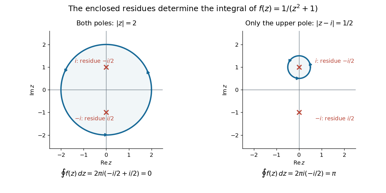
This is the practical appeal of the residue theorem: local Laurent coefficients determine a global contour integral. For a rational function, a few simple pole computations can replace a long parametrized calculation. It also makes real improper integrals accessible by treating the real line as part of a closed contour in the complex plane.

To compute $I={\int }_{-\infty }^{\infty }dx/(1+x^2)$, take $R>1$ and travel along the real line from $-R$ to $R$, then return along the upper semicircle $A_R$, parametrized by $z=R{e}^{it}$ for $0\le t\le \pi$. This contour is positively oriented and encloses the simple pole $i$ only; $-i$ is outside. HenceThe added arc must be controlled before taking a limit. On $A_R$, the reverse triangle inequality gives $|z^2+1|\ge R^2-1$, and the arc length is $\pi R$. The estimation lemma therefore yieldsThe denominator grows quadratically while the arc length grows only linearly. This quantitative comparison, rather than a sketch alone, explains why closing the contour does not alter the limiting real improper integral. It even supplies an error bound: the difference between $\pi$ and the finite real integral is at most $\pi R/(R^2-1)$.

For a numerical check, $R=10$ gives the finite real integral $2\arctan (10)\approx 2.94226$, leaving about $0.19934$ to reach $\pi$. The arc bound is $10\pi /99\approx 0.31733$, comfortably larger than that error. The graph shows both quantities approaching zero. The exact tail here can be checked with the antiderivative $\arctan x$; the residue theorem method remains useful for improper integrals where a convenient real antiderivative is unavailable.

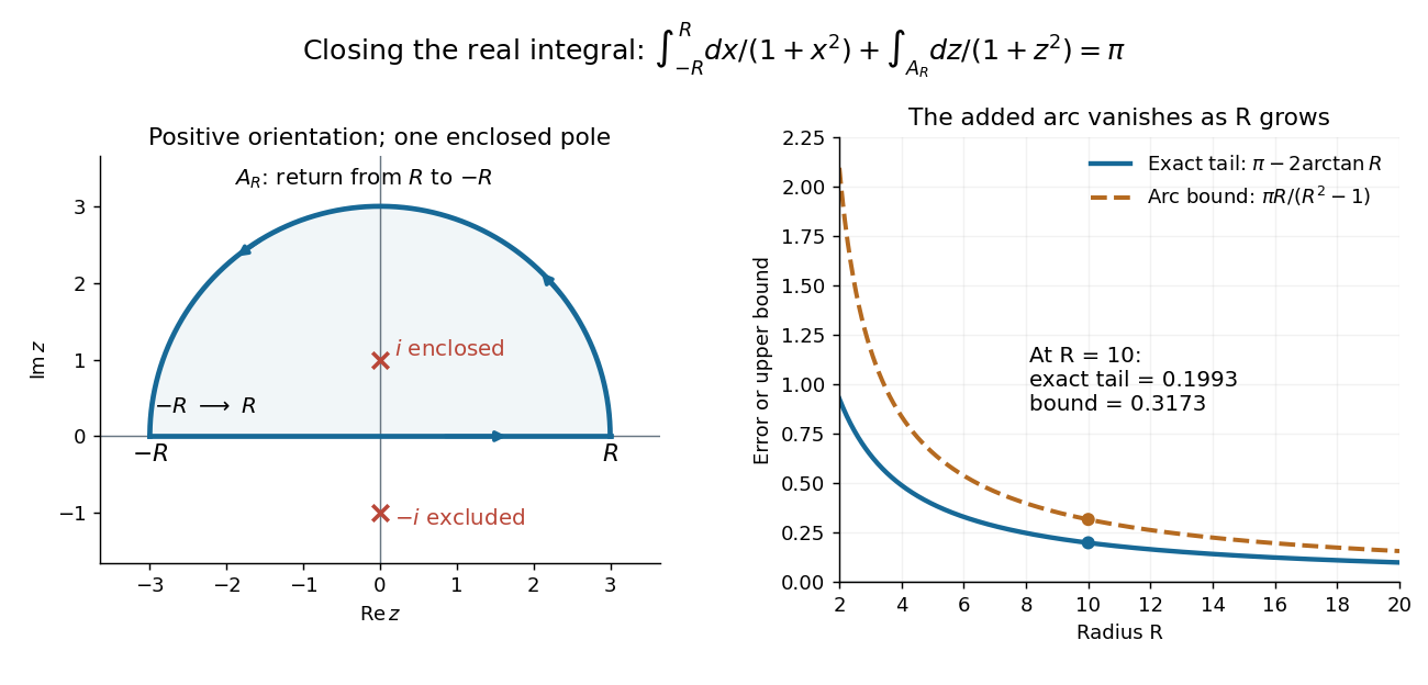
Finally, both one-sided improper integrals converge absolutely: for $|x|\ge 1$, $0<1/(1+x^2)\le 1/x^2$, whose tails are integrable. Thus the symmetric limit computes the ordinary improper integral, not merely a Cauchy principal value, andClosing below instead would enclose the simple pole $-i$. With the same left-to-right traversal of the real line, that contour is clockwise, so its contour integral is $-2\pi i\mathrm{Res}(f,-i)=\pi$ again. This provides a useful sign check: the opposite residue is accompanied by the opposite direction around the enclosed region.

The same strategy extends to many other rational functions: choose a contour, identify its enclosed isolated singularities, compute their residues, and bound the added pieces. The choice of contour and the bound are as much part of the calculation as the residues. ^[ref]

Let $G^{\prime }(z_0)=0$, $G^{\prime \prime }(z_0)\ne 0$, and let $F,G$ be analytic. Assume a contributing contour can be deformed onto two descent arms of the method of steepest descent with one clockwise semicircular avoidance of the pole at $z_0$, and that its other portions are negligible. For the integrand $F(z)e^{-i\lambda G(z)}/(z-z_0)$, a local coordinate with $G-G_0=-i{w}^2/2$ givesThe odd pole term has zero Cauchy principal value on the real arms and integral $-i\pi F_0$ on the clockwise indentation. The constant regular term integrates to $\sqrt{2\pi /\lambda }$ times its coefficient, proving the expansion and generic correction order. A degenerate saddle has a different local width and possibly a different indentation angle; analyticity and a single critical point alone do not imply this result. If $F_0=0$, retain the additive expansion rather than writing asymptotic equivalence to zero.

An integral equation with a kernel singular on the integration contour needs a prescribed limiting interpretation such as a Cauchy principal value. For the Cauchy kernel, the Sokhotski–Plemelj theorem converts a linear scalar equation into a Riemann-Hilbert problem for its two analytic boundary values. Normalization, endpoint regularity and the index of that jump determine homogeneous freedom and solvability.

A singular integral operator has a kernel whose ordinary integral can fail at points on the integration domain. A specified limiting prescription, such as a Cauchy principal value, can still define the operator by cancellation. For the Hilbert transform kernel $1/(t-x)$, subtracting $f(x)$ from a locally Hölder-continuous density leaves $[f(t)-f(x)]/(t-x)$ locally integrable; the constant part is interpreted by symmetric deletion. The limiting prescription and the class of allowed densities are part of the operator's definition, not optional details.

Suppose a contour follows the real axis, closes in the upper half-plane, and avoids each simple real pole $a_j$ by a small semicircle above it. Each indentation is clockwise and tends toIf the large arc vanishes and there are no enclosed poles away from the real axis, the Cauchy principal value is therefore