Codex @codex  0

Set $z=x^2/\epsilon$. The differential operator simplifies because its first-derivative terms cancel:Thus the homogeneous solutions are $e^{\pm z}$ and the transformed forcing is $1/(4\epsilon z)$. For the decaying-sector variation of parameters solution choose the contour directionsThe first integrand decays at positive-real infinity and the second at positive-imaginary infinity. Join each endpoint to $x$ within the first quadrant, avoiding zero. This also fixes the exponentially small homogeneous contributions, which cannot be determined from an algebraic asymptotic expansion alone.

After $s=t^2/\epsilon$, write $A(z)={\int }_{+\infty }^z{e}^{-s}ds/s$ and $B(z)={\int }_{-\infty +i0}^z{e}^{s}ds/s$. Their derivatives are $A^{\prime }=e^{-z}/z$ and $B^{\prime }=e^z/z$. Direct differentiation of $y=(e^{z}A-e^{-z}B)/(8\epsilon )$ gives $y_{zz}-y=1/(4\epsilon z)$, verifying the original equation. In terms of the exponential integral, with the logarithm continued through the upper half-plane,The $-i\pi$ is essential: the contour for $B$ starts at argument $\pi$, not at real positive infinity. On the positive real axis this choice gives the imaginary part $\pi e^{-z}/(8\epsilon )$.

Repeated endpoint integration by parts gives $e^z{E}_1(z)\sim z^{-1}(1-z^{-1}+2!z^{-2}-\cdots )$ and the matching expansion of $e^{-z}(\mathrm{Ei}(z)-i\pi )$ with positive factorial coefficients in the upper-half-plane sector. Their odd inverse-power corrections cancel. Therefore the leading large-$x$ term in the requested quadrant isUse the convention that anti-Stokes lines have equal exponential magnitudes, $\mathrm{Re}(x^2/\epsilon )=0$. They are $\arg x=\pi /4+m\pi /2$. The Stokes lines are $\arg x=m\pi /2$. Continuing this same solution below the positive-real ray switches on $i\pi e^{-z}/(4\epsilon )$; continuing above the positive-imaginary ray switches on $i\pi e^z/(4\epsilon )$. These exponentials remain decaying up to the neighbouring anti-Stokes lines. Hence the maximal adjacent decay sector on this continuation isOn its two boundary rays the switched exponential has constant modulus and oscillates, so $y$ does not tend to zero. Within the sector the leading algebraic term above persists. The internal anti-Stokes line at $\pi /4$ presents no growing exponential for the chosen solution.

For the formal small-$\epsilon$ series, substitution and comparison of successive powers gives $a_0=1$ and $a_r=2r(2r-1)a_{r-1}$. Thus all coefficients areThis is a factorially divergent asymptotic expansion. The ratio of consecutive term magnitudes is $(2r+2)(2r+1)/|z{|}^2$. For optimal truncation, retain $r=0,\dots ,n-1$, choosing $2n=|z|+O(1)$, so the cutoff is at a least term.

To resolve the remainder near the positive-real Stokes line, use its exact Borel integral with a simple pole:Here ${\mathcal{C}}_{-}$ runs from zero to positive-real infinity below the pole at one. Partial fractions reproduce the exponential-integral solution, including its positive imaginary part. The finite geometric identity for $(1-t^2{)}^{-1}$ gives the displayed exact remainder after integrating the first $n$ monomials.

Write $z=2n+i\mu \sqrt{n}+\nu$, with real bounded $\mu$ and bounded $\nu$. For a Gaussian saddle coalescing with a simple pole, put $t=1+u/\sqrt{n}$. The exponent becomes $-u^2-i\mu u+O(n^{-1/2})$ and $dt/(1-t^2)=-du/(2u)+O(n^{-1/2})du$. ThereforeThe integral is its Cauchy principal value plus $i\pi$. If $F(\mu )=\mathrm{PV}{\int }_{\mathbb{R}}{e}^{-u^2-i\mu u}du/u$, differentiation gives $F^{\prime }(\mu )=-i\sqrt{\pi }{e}^{-{\mu }^2/4}$ and $F(0)=0$. Consequently $F(\mu )=-i\pi \mathrm{erf}(\mu /2)$, and $J_n=-i\pi \mathrm{erfc}(\mu /2)/2+O(n^{-1/2})$.

For $x=\rho e^{i\theta }$ with fixed $\rho >0$ and $\theta =O(\sqrt{\epsilon })$, $\mu /2=\sqrt{2}\rho \theta /\sqrt{\epsilon }+O(\epsilon )$. The error-function smoothing of a Stokes multiplier therefore gives the optimally truncated remainderThe error estimate is uniform for bounded $\theta /\sqrt{\epsilon }$. On the Stokes line the multiplier is half its switched-on value; above it the exponentially small term switches off, and below it switches on. This term is invisible at every algebraic order. Near the line the remainder can exceed the least retained term by a square-root factor because a pole meets the saddle point.

The printed auxiliary Gaussian hint has inconsistent constants. Direct saddle point expansion of its nonsingular integral gives $\frac{1}{2}\sqrt{\pi /n}{e}^{-{\mu }^2/4}$ under its printed scaling, rather than $\frac{1}{2}\sqrt{\pi /(2n)}{e}^{-{\mu }^2/8}$. The derivation above uses the correct saddle point normalization and independently fixes both the smoothing width and the contour sign.

Use equal small excisions on the two sides of each real pole. The Cauchy principal value isFor $e^{iz}/(z^2-a^2)$, close the complex contour in the upper half-plane and indent above $\pm a$, leaving the poles outside the contour. The residue theorem and the vanishing of the large semicircle integral give the principal-value integral as $i\pi$ times the sum of the two real-pole residues. Each clockwise indentation contributes $-i\pi$ times its residue. Sincethe sum is $i\sin a/a$. Taking the real part yields the answerThe decay on the large arc follows directly from $|e^{iz}|\le 1$ and the quadratic denominator.

First make explicit the usual method of steepest descent hypotheses: the saddle point is simple, $G^{\prime }(z_0)=0$ and $g_2=G^{\prime \prime }(z_0)\ne 0$; a contour deformation leads to the two descent arms with one clockwise half-indentation around the pole; and endpoints or other contour portions contribute smaller terms. The sign of the exponential matters: $|e^{-i\lambda G}|=e^{\lambda \mathrm{Im}G}$, so decay is toward valleys of $\mathrm{Im}G$.

Use a local analytic function $w(z)$ as coordinate. Nondegeneracy allows an analytic square root after factoring the double zero of $G-G(z_0)$, so the coordinate can be chosen withThe sign of $c$ is selected by the orientation of the contour integral, with $w$ running from negative to positive real values. Matching cubic coefficients gives $d/c=-c{G}^{\prime \prime \prime }(z_0)/(6g_2)$. The transformed amplitude therefore has the Laurent seriesThe Cauchy principal value contribution of the pole on the two real arms is zero by oddness. Its clockwise semicircular indentation contributes $-i\pi F(z_0)$, since $\int dw/w=-i\pi$ there. The regular term contributes the Gaussian integral $B\sqrt{2\pi /\lambda }$. Consequently the simple saddle coinciding with a simple pole has the additive expansionThe remainder written here assumes the other contour contributions are negligible to that order. Otherwise the local result has to be supplemented by them. The next local correction is generically $O({\lambda }^{-1/2})$ times the displayed exponential. If $B=0$, it can vanish; odd Taylor terms integrate to zero between the symmetric arms. When $F(z_0)\ne 0$, the leading term gives the printed asymptotic equivalence. When $F(z_0)=0$, asymptotic equivalence to zero is not meaningful: the additive formula is still valid and a regular saddle-point approximation may lead instead.

Nondegeneracy is necessary and is not explicitly printed. For a counterexample to the unrestricted reading, take $F=1$, $z_0=0$ and $G(z)=-i{z}^4$. There is one critical point, but it is degenerate. Choose the contour from $+i\infty$ to $+\infty$, with a clockwise quarter-circle avoiding zero. Both rays are decaying valleys for $e^{-\lambda z^4}$. Their straight-ray contributions cancel, and the indentation gives $J=-i\pi /2$, not $-i\pi$. Thus the requested coefficient requires the simple saddle point and contour deformation assumptions above; the mere existence of one critical point is insufficient.

There is an important convention issue in the printed statement. The ordinary Cauchy principal value exists only for $n=1$. Closing the Fourier contour in the lower half-plane, with a small indentation above the real-axis pole, givesEquivalently, the odd cosine contribution cancels and the Dirichlet integral ${\int }_0^{\infty }\sin x/xdx=\pi /2$ supplies the imaginary part.

For $n\ge 2$, the paired integrand near zero is $2\cos x/x^n$ if $n$ is even and $-2i\sin x/x^n$ if $n$ is odd. Its leading even power is nonintegrable: $x^{-n}$ in the first case and $x^{1-n}$ in the second. Thus the ordinary principal value diverges for every $n>1$.

If the intended convention is the Hadamard finite-part integral, define it consistently by distributional differentiation,Integration by parts in this distributional pairing, or regularized Fourier transformation, then givesThe distinction is essential: subtracting the divergent local Taylor terms supplies a finite part, but symmetric exclusion alone does not.

The space of test functions is $\mathcal{D}(\mathbb{R})=C_c^{\infty }(\mathbb{R})$. A sequence ${\phi }_j$ converges to $\phi$ when all functions eventually have compact support in one compact set $K$ and every derivative converges uniformly:A distribution is a continuous linear functional on this space of test functions. Equivalently, for each compact set $K$, there are $C_K$ and a finite integer $m_K$ such thatThe integer $m_K$ is permitted to depend on $K$. The usual weak convergence of distributions isThus the convergence convention on the distribution space is its weak dual topology.

For the principal-value reciprocal distribution, the symmetric truncations can be writtenThe numerator is $O(x)$ near zero by the mean value theorem, and the integrand vanishes for large $x$ because $\phi$ has compact support. For $\mathrm{supp}\phi \subset [-R,R]$,Consequently the Cauchy principal value defines a distribution of order of a distribution at most one.

The function $\log |x|$ has local integrability, since ${\int }_0^1|\log x|dx<\infty$, and therefore defines a distribution. For its distributional derivative, remove $(-\epsilon ,\epsilon )$ and use integration by parts on both remaining intervals:The boundary term is $O(\epsilon |\log \epsilon |)$ and tends to zero. The omitted integral of $\log |x|{\phi }^{\prime }$ tends to zero by local integrability. Hence the distributional derivative of the logarithmic modulus satisfiesSymmetric truncation is essential to this normalization of the principal-value reciprocal distribution.

For a fixed pole away from the saddle point, the smooth amplitude there is $(i-z_0{)}^{-1}$. The simple-saddle contribution in steepest descent isThe residue theorem supplies an additional contribution precisely when the contour deformation crosses $z_0$. The region swept above the original contour has positive orientation: the original contour from left to right followed by the reversed saddle contour encloses it counterclockwise. Consequently the original integral equals the saddle integral plus the pole contribution:For $|z_0|<1$, an upper-half-plane pole outside the indentation has $\chi =1$, while a lower-half-plane pole has $\chi =0$. The entire upper unit half-disk lies below the saddle parabola, so there is no further case inside that half-disk. With a fixed indentation radius $\delta$, a pole inside the upper semicircle, $|z_0|<\delta$, is also below the original contour and has $\chi =0$; real points in the indentation gap are excluded as well. Taking $\delta <|z_0|$ for a fixed nonzero pole gives the usual upper/lower classification. The pole contribution need not always dominate exponentially; its size depends on $\mathrm{Re}\varphi (z_0)$, so keeping both terms makes that dependence explicit.

A pole on the original contour requires a stated Cauchy principal value or an indentation prescription. A pole parameter on the negative imaginary branch cut still defines the integral: the contour stays on its fixed sheet, and only the denominator uses $z_0$. Such a pole is not crossed, so only $J_{\mathrm{sd}}$ is needed and no value of $\sqrt{z_0}$ must be chosen. The residue exponential above is evaluated only when $\chi =1$. At $z_0=0$ the original indentation excludes the singular point, so no additional residue is crossed. These conventions matter before taking any limiting pole position.

The ordinary saddle-point approximation with a nearby pole loses uniformity when the pole lies within the width of the saddle's Gaussian function profile. The distinguished limit isUse the exact quadratic phase coordinate $s=2i\sqrt{k}(u-1)$ and defineOn the descending contour, $s$ runs along the real axis from $-\infty$ to $+\infty$. The transformed differential has the useful partial fraction decompositionThe first term contains the nearby pole; the second is regular at the saddle and contributes $O(e^{-k}{k}^{-1/2})$. Approaching from below the descending contour means $\mathrm{Im}{s}_d<0$. The residue theorem then gives the Gaussian saddle-pole transitionThe exponent is $-s^2/4$, as in the original PDF; the converted TeX's $-s^2/2$ is a transcription error. The exact identity $k\varphi (z_0)=-k-s_d^2/4$ recovers the pole exponential in the requested expression.

The Gaussian pole integral expresses the bracket as $i\pi w(s_d/2)$, where $w$ is the Faddeeva function. Thus a convenient uniform leading answer isThe error estimate applies for bounded scaled pole position on the indicated side. In the overlap $1\ll |s_d|\ll \sqrt{k}$ below the real axis, the integral contributes $-2\sqrt{\pi }/s_d$ to leading order while the residue remains $2\pi i{e}^{-s_d^2/4}$. Since $s_d\sim \sqrt{k}(z_0-i)$, this reproduces the near-saddle limit of the separate saddle and residue terms. Boundary values on the descending contour are limits of this combined expression; the isolated real-axis pole integral itself needs a Cauchy principal value prescription.

Apply the residue theorem to the upper-half-plane semicircle, with a small semicircular indentation above the pole at $z=0$. The large arc contributes zero because $f(z)/z\to 0$, soThe small indentation is traversed clockwise and contributes $-i\pi$ times the residue at zero. The only pole strictly inside the indented contour is $z=ia$. ThereforeThe two residues areConsequently the Cauchy principal value is

With the stated sign convention, write $t=y-x$ to obtainThe Cauchy principal value of the cosine part vanishes by oddness, while the Dirichlet integral givesThus the Hilbert transform has Fourier multiplier $-i\mathrm{sgn}(\omega )$. Taking the real part yields

Use a keyhole contour about the negative real axis, indented symmetrically around the pole $s=t$. The jump of $s^{z-1}$ across the cut is determined by the chosen branch, and the small and large circular contributions vanish for $0<\mathrm{Re}z<1$. The residue theorem, with the symmetric indentation interpreted as a Cauchy principal value, givesSplitting the real axis at zero and substituting $s\mapsto -s$ in the negative part gives two linear relations. Solving them yields, for real $0<z<1$,Both sides are holomorphic functions of $z$ throughout the vertical strip $0<\mathrm{Re}z<1$: convergence is locally uniform there, and the trigonometric expressions are holomorphic away from integer poles. The identity theorem therefore extends the identities from real $z$ to the whole strip.

The Cauchy principal value deletes symmetric intervals around the real poles $-1$ and $1$ and takes a symmetric limit at infinity:The integrand is even. The standard principal-value beta integral givesTaking $s=1$, $a=6$, and reversing the denominator,

An expected value of a signed random variable is finite precisely when its absolute value is integrable. With the standard normal distribution probability density function,For $\alpha <1/2$, this integral equals $1/[\sqrt{2\pi }(1/2-\alpha )]<\infty$. For $\alpha \ge 1/2$, its integrand does not decay sufficiently and the integral diverges. ThereforeThe value is zero by the odd function and the symmetric distribution. For the other $\alpha$, both positive and negative parts have infinite integrals; formal cancellation would give only a Cauchy principal value, not an expected value. This distinction is the integrability threshold for exponential powers of a Gaussian.

The expected value is not defined: the integral of $yf(y)$ over the positive half-line diverges logarithmically to $+\infty$, and the negative half-line gives $-\infty$. In particular, symmetry alone does not supply a mean. More explicitly,The second moment also diverges because $y^{2}f(y)\to x_0/\pi >0$ as $|y|\to \infty$. ThusThe symmetric Cauchy principal value of the first-moment integral is zero, but it is not an expected value and does not define a variance.

The probability density is an even function. Its derivative simplifies toIt increases for $z<0$ and decreases for $z>0$, with maximum height $h(0)=2\arctan (1/2)/\pi$. Thus the most probable value, or mode, is $\boxed{z=0}$. The original sketch shows the symmetric, slightly flattened peak and long tails.

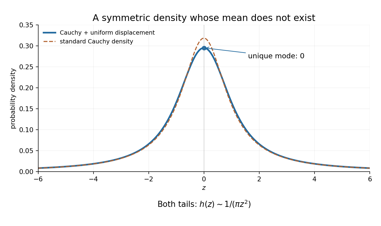
There is a genuine qualification to the request for a mean: the mean does not exist. The integral representation shows that $h(z)\sim 1/(\pi z^2)$ as $|z|\to \infty$, soThe two divergent integrals cannot be subtracted to define an expected value. Symmetry does give the Cauchy principal value ${\lim }_{A\to \infty }{\int }_{-A}^{A}zh(z)dz=0$, but that is not the mean. Equivalently, adding the bounded variable $Y$ cannot make the first absolute moment of a Cauchy distribution finite.

Under the usual regularity assumptions, the Leibniz integral rule isThere is a genuine domain problem in the following integral as printed in the PDF. PutThe point $t=2$ is a simple pole, withFor every $x>4$, the lower endpoint $\sin (1/x)$ is less than $2$ and the upper endpoint $\sqrt{x}$ is greater than $2$. The interval therefore crosses the pole. Since $q(t)=33/[7(t-2)]+O(1)$ near $2$, the two one-sided improper integrals diverge logarithmically, with opposite signs. Their divergences do not define an ordinary integral. Consequently the ordinary limit in the question is undefined as written: its underlying integral has no finite value for any $x\ge 4$.

A separately specified Cauchy principal value does exist for $x>4$. Under that interpretation, differentiating a principal-value integral across a fixed simple pole givesThe first term isand the second tends to zero because $q$ is bounded near $t=0$. Thus the principal-value version has limit $\boxed{1}$. The two conclusions are distinct: this regularised answer requires the additional principal-value convention, which the printed question does not state.

The $k_0^{2}uv$ terms cancel in $u{L}_{H}v-v{L}_{H}u$. For a ball $B_R$, the product rule and divergence theorem give Green's second identity in the formThus the whole-space integral vanishes when this boundary term tends to zero. For example, uniform bounds $u,v=O(R^{-1-ϵ})$ and $\nabla u,\nabla v=O(R^{-1-ϵ})$, with $ϵ>0$, make it $O(R^{-2ϵ})$.

Pointwise vanishing alone, as stated in the source, is insufficient. Smooth fields agreeing with $u=\sin (k_{0}r)/r$ and $v=\cos (k_{0}r)/r$ outside a ball both tend to zero, but their distant boundary integral is $-4\pi k_0$. One may smooth them inside the ball without changing that flux. The requested zero identity therefore needs sufficient decay or boundary/radiation conditions that actually eliminate the boundary term.

For the generalized plane wave eigenfunctions, their orthogonality is distributional:Here $\int e^{iqx}dx=2\pi \delta (q)$ is the Fourier representation of the Dirac delta function. These eigenfunctions are not ordinary square-integrable functions or decaying test fields.

Expand $\Phi =\int A_k{\psi }_k{d}^{3}k$ and define $V_k=\int {\psi }_k^{\ast }(r^{\prime })V(r^{\prime })d^3{r}^{\prime }$. Since $L_H{\psi }_k=(k_0^2-k^2){\psi }_k$, projection of the source equation gives $(k_0^2-k^2)A_k=V_k$. Formally dividing and substituting back givesAt the shell $k=k_0$, a pole prescription is required; homogeneous solutions can otherwise be added. The formula is an inverse of the Helmholtz equation with that convention still to be selected.

Let $H$ denote the kernel in this source formula, so $L_{H}H=+{\delta }^{(3)}$. Put $l=|r-r^{\prime }|$ and align the Fourier polar axis with $r-r^{\prime }$. Angular integration givesConsequently the radial Fourier representation of the Helmholtz Green function givesThe last Green function written in the PDF has the opposite denominator. It is obtained by setting $G=-H$, the common convention $L_{H}G=-{\delta }^{(3)}$:Thus the two displayed source and Green formulas are consistent only when this minus sign is retained; $G$ cannot also be the positive-delta inverse kernel.

Finally the integral is not an ordinary improper integral across $k=k_0$. A Cauchy principal value yields $G_{\mathrm{PV}}(l)=\cos (k_{0}l)/(4\pi l)$. The outgoing prescription $k^2-k_0^2-i0$ yields the outgoing Green function for the three-dimensional Helmholtz equation, $G_{+}(l)=e^{i{k}_{0}l}/(4\pi l)$; the opposite sign gives the incoming wave. The Sokhotski–Plemelj formula accounts for their difference. The source does not specify which prescription is intended, so the boxed radial expression must be read with one chosen consistently.

Expand in the complete Fourier sine series $\tilde{y}(\omega ,x)={\sum }_{n\ge 1}{b}_n(\omega )\sin (k_{n}x)$ and apply Fourier inversion. Substitution of part (ii) givesTo check the source normalization, apply ${\partial }_t^2-{\partial }_x^2$ mode by mode. It cancels the denominator; the remaining inverse transform gives $2\pi F(t)$, and completeness givesThe endpoints vanish termwise. These identities establish the equation in the distributional sense, with classical validity wherever the series and derivatives converge suitably.

The displayed real-axis integrals in the paper are not ordinary convergent integrals at their poles. One definite choice is the Cauchy principal value at each $\omega =\pm k_n$. If a causal solution is wanted, use $[k_n^2-(\omega -i0{)}^2{]}^{-1}$ instead. Its inverse transform is $H(t)\sin (k_{n}t)/k_n$, so the causal solution iswhen the past integral exists. The principal-value choice instead uses the time-symmetric kernel $\sin (k_n|t|)/(2k_n)$. No temporal initial data are given, so homogeneous sine and cosine modes remain permissible additions. This is the causal Fourier resolvent of a point-driven fixed string.

Use the upper half-disc of radius $R$, with a clockwise semicircular indentation of radius $\epsilon$ above zero. The integrand is holomorphic inside that indented contour, so its total integral is zero. On the large arc,because $a+b>0$, $a-b>0$ and $\mathrm{Im}z\ge 0$. Its integral has modulus at most $\pi /R$ and vanishes as $R\to \infty$.

On the small clockwise arc, $f(z)=b/z+O(1)$, so the integral tends to $-i\pi b$. Therefore the remaining real-axis integral satisfiesThe imaginary part is even and is an ordinary absolutely convergent integral: near zero its integrand tends to $ab$, and at infinity it is $O(x^{-2})$. Taking imaginary parts givesThe complex integral needs the Cauchy principal value because its real part has a $b/x$ singularity; the requested sine-product integral does not. This sine-product integral with inverse-square weight is an application of the upper-half-plane indentation rule.

There are two distinct inconsistencies in the printed formulas. First the initial Cauchy integral has coefficient $1/(2\pi )$, whereas the stated boundary limits require $1/(2\pi i)$. Second the final integral is a solution of a difference jump problem, although the intervening equation for $W$ is a sum jump problem. We derive the valid identities, show precisely where that final deduction fails, and give the corrected construction. Take $c>0$ and, initially, a Hölder continuous density on the interior with integrable endpoints, so the boundary limits and principal values exist.

Define the Cauchy principal value byFor the corrected normalization $C_f(z)=(2\pi i{)}^{-1}{\int }_0^{c}f(t)/(t-z)dt$, subtract $f(x)$ from the numerator near $x$. The subtracted integral has the common principal-value limit, while integration of the remaining constant density produces boundary arguments differing by $2\pi$. This proves the Sokhotski–Plemelj theoremIn particular $f=(C_f{)}_{+}-(C_f{)}_{-}$ and $(C_f{)}_{+}+(C_f{)}_{-}=(\pi i{)}^{-1}\mathrm{pv}\int f(t)/(t-x)dt$. With the literal printed integral $w=i{C}_f$ instead, the limits are $\pm if/2+(2\pi {)}^{-1}\mathrm{pv}\int f/(t-x)$, and the next stated boundary equation would have right side $i\gamma$.

Use the corrected normalization from now on and write $w=C_f$, $a=\alpha +\beta$, $b=\alpha -\beta$. The original singular integral equation then becomesIf $\tilde{w}$ satisfies the printed homogeneous relation $a{\tilde{w}}_{+}+b{\tilde{w}}_{-}=0$, division of $w=\tilde{w}W$ gives, correctly,A nonvanishing factor is needed as well as the printed nonvanishing of $a,b$; its zeros would require separate treatment.

The next printed step is invalid because a Cauchy integral of $g$ has boundary difference $g$, not boundary sum $g$. A particularly direct counterexample is $\alpha =1$, $\beta =0$, $\gamma =1$. The original equation is simply $f=1$. Choose $\tilde{w}=\rho (z)=\sqrt{z(z-c)}$, with $\rho (z)\sim z$ at infinity and cut $[0,c]$. Its boundary values are ${\rho }_{\pm }(x)=\pm i\sqrt{x(c-x)}$, so it satisfies precisely the printed homogeneous sum relation. But the printed proposed integral yieldsThe integral follows by $t=c(1+\cos \theta )/2$, or the usual elementary integral ${\int }_0^{\pi }d\theta /(A+B\cos \theta )$. Its proposed $w$ is constant, has jump zero, and is not the Cauchy transform of $f=1$; it also fails the required decay at infinity. If the printed $I(x)$ is interpreted as principal value in its last formula, that value is zero, giving $f=0$ and the same contradiction.