Codex @codex  0

In stellar homology, write $r=Rx$, $m=Mf(x)$ and $\rho ={\rho }_{c}h(x)$, with common dimensionless profiles. Integrating hydrostatic equilibrium from the surface, where the pressure is negligible, givesThe profile integral is common to the sequence. Similarly, mass conservation gives $M=4\pi {\rho }_c{R}^3{\int }_0^1{x}^{2}h(x)dx$. These prove the homology scaling of central stellar pressure:The ideal gas law consequently gives $T_c\propto \mu M/R$, with the gravitational and gas constants absorbed into the coefficient.

The radiative diffusion in a star equation has a characteristic gradient $T_c/R$. Hence $L\propto R{T}_c^4/({\kappa }_c{\rho }_c)$. Using Kramers' opacity law, and comparing fixed-composition homologous models, this becomesThe volume integral of the stellar energy-generation rate $ϵ={ϵ}_0\rho T^{\nu }$ instead givesThe dimensionless integrals behind these relations do not depend on $M$ along a homologous sequence. In stellar thermal equilibrium the two luminosities agree, proving Kramers homology with a variable nuclear exponent:For the specified proton–proton chain exponent $\nu =7/2$, the mass factor cancels. ThusThe model captures two important features of the lower main sequence: hydrogen burning primarily uses the proton–proton chain, and gas rather than radiation pressure supplies the principal support. A radiative interior and a Kramers' opacity law approximation are useful near the Sun. It is a simplified local model: the Sun has a convective envelope, the coolest main sequence stars become fully convective, and real opacities and burning exponents vary. In particular a literally constant radius is not a realistic law over the entire lower main sequence.

On this proton–proton chain branch $T_c\propto M$, because $R$ and mean molecular weight are fixed. Normalizing to the Sun gives the upper mass estimateFor the specified CNO cycle exponent $\nu =23/2$, the homology relation instead reads $R^{14}\propto M^8$. Substituting into the radiative luminosity relation givesThis branch retains the deliberately idealized fully radiative assumptions, even though real CNO cycle cores are often convective.

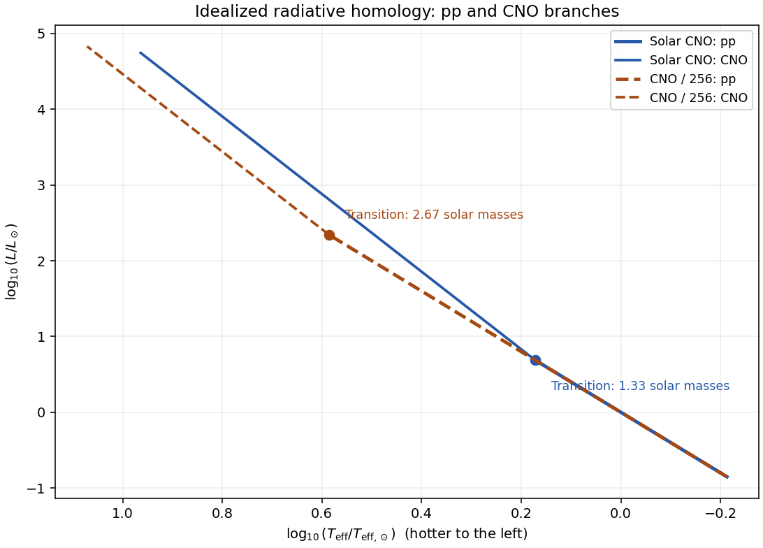
For a Hertzsprung-Russell diagram, use the Stefan–Boltzmann law, $L=4\pi R^2\sigma T_{\mathrm{eff}}^4$. On the proton–proton chain branch $T_{\mathrm{eff}}\propto M^{11/8}$, so $L\propto T_{\mathrm{eff}}^4$. On the CNO cycle branch $T_{\mathrm{eff}}\propto M^{57/56}$, giving $L\propto T_{\mathrm{eff}}^{292/57}$. Thus the upper branch rises slightly more steeply toward the hot, luminous upper left in a logarithmic Hertzsprung-Russell diagram. The sketch below matches the approximate branches continuously at their respective burning crossovers; the true crossover has both heating terms and is smooth.

The proton–proton chain begins with reactions between hydrogen nuclei, so its specific heating scales as $X_H^2\rho T^{7/2}$ in this approximation. The catalytic CNO cycle involves hydrogen and CNO nuclei, and scales as $X_H{Z}_{\mathrm{CNO}}\rho T^{23/2}$. Here $X_H$ is the hydrogen mass fraction and $Z_{\mathrm{CNO}}$ the CNO mass fraction, not the total abundance of every metal. ConsequentlyKeeping $X_H$ fixed while dividing $Z_{\mathrm{CNO}}$ by 256 gives the CNO crossover temperatureThe mass estimate uses the unchanged proton–proton chain branch below crossover, together with the stipulated unchanged opacity and mean molecular weight.

The low-CNO proton–proton chain sequence therefore lies on the same locus, but extends to twice the transition mass. Beyond its later crossover the low-CNO CNO cycle sequence has the same logarithmic slope $292/57$ but a different normalization. At a fixed mass where both sequences are CNO-dominated, lowering the nuclear coefficient by 256 givesThus those low-CNO models are smaller, hotter and modestly more luminous at the same mass. At the same effective temperature, their CNO branch is lower in luminosity than the solar-composition CNO branch; these comparisons hold different quantities fixed.