Codex @codex  0

The improper integral converges: its integrand is bounded near zero and at most $x^{-n}$ for $x\ge 1$, which is integrable because $n\ge 2$.

Set $\theta =\pi /n$, $\omega =e^{2i\theta }$ and $\zeta =e^{i\theta }$. Apply the residue theorem to $F(z)=1/(1+z^n)$ on the positively oriented sector contour consisting of the segment $0\to R$, the arc $R{e}^{it}$ for $0\le t\le 2\theta$, and the segment $R\omega \to 0$, with $R>1$. No pole lies on the boundary. Exactly one root of $z^n=-1$ is inside this sector, namely $\zeta$; it is a simple pole. Part (a) givesOn the returning ray, put $z=\omega x$ with $x$ decreasing from $R$ to zero. Since ${\omega }^n=1$, the two ray contributions areOn the arc, $|1+z^n|\ge R^n-1$, so the estimation lemma bounds its contour integral byThe residue theorem and the convergence already established now giveUsing $1-e^{2i\theta }=-2i{e}^{i\theta }\sin \theta$, we concludeThe sector also works for $n=2$, when it is the upper semicircle. Its angle is chosen so that $z^n$ has the same value on the two rays.

The Heisenberg picture evolution of the annihilation operator follows from $[H,a_{\mathbf{p}}]=-E_{\mathbf{p}}{a}_{\mathbf{p}}$. With $p^0=E_{\mathbf{p}}$, this gives the mode expansion of a free fieldDefine ${\Delta }^{+}(z)={\int }_{\mathbf{p}}{e}^{-ip\cdot z}/(2E_{\mathbf{p}})$. The time-ordered product then gives the Feynman propagatorThe last expression follows by closing the $p^0$ contour integral below for $z^0>0$ and above for $z^0<0$; the scalar Feynman propagator pole prescription supplies the required positive- and negative-frequency terms.

For $z^0\ne 0$ every term obeys the homogeneous Klein-Gordon equation. At $z^0=0$, the equal-time commutator of the fields vanishes, so the propagator is continuous and there is no derivative of a Dirac delta function. Its first time derivative has the jumpThe second time derivative therefore supplies precisely the source:Thus the defined Feynman propagator is a Green's function with source normalization $-i$; $i{\Delta }_F$ has source normalization $+1$. Keeping this factor avoids confusing the vacuum expectation value convention with conventions which define the propagator after dividing by $i$.^[ref]

Cauchy's integral theorem states that a holomorphic function on a simply connected open region has zero contour integral around every closed piecewise smooth contour in that region. More generally the same holds for a contour homologous to zero in its domain of holomorphy. Having no singularity on the curve alone is insufficient: $1/z$ has a nonzero contour integral around the unit circle.

Put $z=e^{i\theta }$, so $d\theta =dz/(iz)$, $\cos 2\theta =(z^2+z^{-2})/2$ and ${\cos }^{2}3\theta =(z^6+2+z^{-6})/4$. The contour integral isThe enclosed poles are $0$ and $\pm 1/\sqrt{2}$. For the rational function displayed without the prefactor $1/(4i)$, the residue at zero is $-21/8$ and the two other residues sum to $27/8$. Therefore the residue theorem givesA useful independent check is the Fourier series $(5-4\cos \varphi {)}^{-1}=\frac{1}{3}[1+2{\sum }_{k\ge 1}{2}^{-k}\cos k\varphi ]$; only its constant and third Fourier coefficients survive.

Use the branch cut $[-1,1]$ and the branch of a multivalued function normalized by $\sqrt{z^2-1}\sim z$. The Laurent series from the preceding solution has $z^{-1}$ coefficient $3/8$. Consequently every sufficiently large positively oriented circle givesAlthough $f$ grows cubically, its other Laurent series terms have zero contour integral. Choosing the opposite branch of a multivalued function reverses the sign; neither the branch of a multivalued function nor the orientation can be omitted from the answer.

Parametrize the positively oriented unit circle by $z=e^{i\theta }$. Then $dz=izd\theta$ andConsequently the contour integral already evaluated satisfies

On the upper semicircular contour, $|z|=R$ and the reverse triangle inequality gives $|z^4+1|\ge R^4-1>0$. Its arc length is $\pi R$, so the estimation lemma givesThe arc is open, so an ordinary integral sign is appropriate even though the source uses a closed-integral symbol there. Subtracting the vanishing arc contribution from the closed contour integral gives the real-line improper integral $\pi /\sqrt{2}$. Its integrand is an even function, and its tail is $O(x^{-2})$, ensuring convergence. Thus

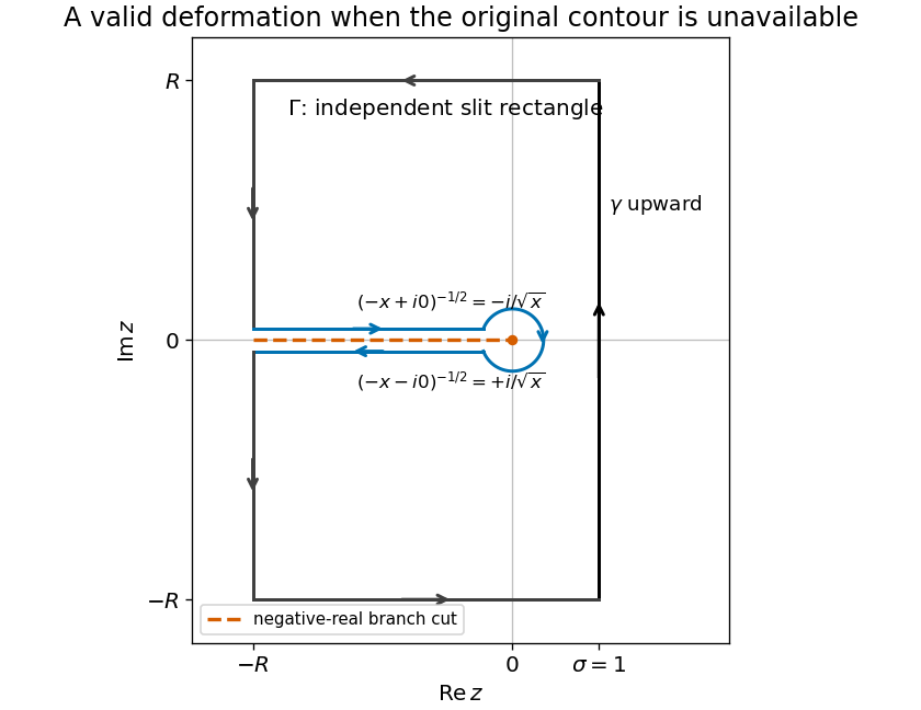
On the small clockwise contour $z=ϵe^{i\theta }$, $\theta$ decreases from $\pi$ to $-\pi$. Uniformly on that arc, $e^{z-\sqrt{z}}=1+O(\sqrt{ϵ})$, and henceThe large arcs also vanish. To make this precise for the displayed geometry, take them on the left semicircle $z=\gamma +R{e}^{i\theta }$, $\pi /2\le \theta \le 3\pi /2$, split at the cut. On the principal holomorphic branch, $\mathrm{Re}\sqrt{z}\ge 0$, $|z|\ge R-\gamma$, and $\mathrm{Re}z=\gamma +R\cos \theta$. The estimation lemma givesFor the last bound, symmetry and $\sin u\ge 2u/\pi$ on $0\le u\le \pi /2$ imply that the angular integral is at most $\pi /R$. The exact choice of large arcs does not affect the limiting result. The vertical improper integral converges absolutely because $e^{-\mathrm{Re}\sqrt{\gamma +iy}}/|\gamma +iy|$ decays as $O(e^{-c\sqrt{|y|}}/|y|)$.

Taking limits in the closed contour integral now yields $2\pi iJ+2iK-2\pi i=0$, where $K={\int }_0^{\infty }{e}^{-x}\sin (\sqrt{x})dx/x$. ThusAs an optional explicit evaluation, put $x=t^2$ and define $K(a)=2{\int }_0^{\infty }{e}^{-t^2}\sin (at)dt/t$. Differentiation under the integral sign and the Gaussian integral give $K^{\prime }(a)=\sqrt{\pi }{e}^{-a^2/4}$ and $K(0)=0$. Therefore $K=K(1)=\pi \mathrm{erf}(1/2)$ and $J=\mathrm{erfc}(1/2)\simeq 0.479500$ in terms of the error function and complementary error function.

Cauchy's integral theorem states that a holomorphic function on a simply connected open region has zero contour integral around every closed piecewise smooth contour in that region. More generally the same holds for a contour homologous to zero in its domain of holomorphy. Having no singularity on the curve alone is insufficient: $1/z$ has a nonzero contour integral around the unit circle.

Put $z=e^{i\theta }$, so $d\theta =dz/(iz)$, $\cos 2\theta =(z^2+z^{-2})/2$ and ${\cos }^{2}3\theta =(z^6+2+z^{-6})/4$. The contour integral isThe enclosed poles are $0$ and $\pm 1/\sqrt{2}$. For the rational function displayed without the prefactor $1/(4i)$, the residue at zero is $-21/8$ and the two other residues sum to $27/8$. Therefore the residue theorem givesA useful independent check is the Fourier series $(5-4\cos \varphi {)}^{-1}=\frac{1}{3}[1+2{\sum }_{k\ge 1}{2}^{-k}\cos k\varphi ]$; only its constant and third Fourier coefficients survive.

Use the branch cut $[-1,1]$ and the branch of a multivalued function normalized by $\sqrt{z^2-1}\sim z$. The Laurent series from the preceding solution has $z^{-1}$ coefficient $3/8$. Consequently every sufficiently large positively oriented circle givesAlthough $f$ grows cubically, its other Laurent series terms have zero contour integral. Choosing the opposite branch of a multivalued function reverses the sign; neither the branch of a multivalued function nor the orientation can be omitted from the answer.

TODO: the original closed-contour drawing is absent from the source. The following independent Bromwich contour deformation establishes the required discontinuity relation without asserting the missing drawing's exact geometry. Orient the vertical line upward, as required by the positive imaginary answer in the next part, and use the principal square root, $-\pi <\arg z<\pi$.

Close a truncated vertical line to the left with a rectangle, slit it along the negative real axis, and exclude a small circle about zero. The integrand is holomorphic inside that slit domain, so the boundary contour integral is zero. Horizontal boundary integrals are $O(R^{-1/2})$: integrating $e^x$ along $-R\le x\le 1$ gives a bounded factor while $|z{|}^{-1/2}\le R^{-1/2}$. The left boundary contributes $O(e^{-R}{R}^{1/2})$, and the small circle contributes $O(\sqrt{\epsilon })$. All vanish in the indicated limits.

At $z=-x$ with $x>0$, the upper and lower bank values are respectively $-i{e}^{-x}/\sqrt{x}$ and $+i{e}^{-x}/\sqrt{x}$. The boundary follows the upper bank toward zero and the lower bank away from zero. Their combined contribution is $-2i{\int }_0^{\infty }{e}^{-x}{x}^{-1/2}dx$. HenceThe vertically improper integral converges conditionally; these estimates also justify the contour limit. Reversing the vertical orientation reverses its sign.

Use the positive orientation shown in the source: the upper bank runs outwards and the lower bank returns towards one. On those banks the logarithm branch has values $\ell -i\pi$ and $\ell +i\pi$, respectively, with $\ell =\log (x-1)$. Their squared difference is $-4i\pi \ell$. The residue theorem therefore givesand henceThe large-circle contribution is $O(R^{-2}{\log }^{2}R)$ and the small circle about one contributes $O(\epsilon |\log \epsilon {|}^2)$, both tending to zero. These estimates justify replacing the closed contour integral by its two cut-bank integrals.

Take $g(z)=L(z{)}^3/z^3$ on the same logarithm branch. At zero, $L(z{)}^3=-z^3+O(z^4)$, so the apparent singularity is removable and the closed contour integral is zero. The bank difference isThe circular contributions vanish by the previous estimates with the third power of the logarithm. ConsequentlyThe last integral is $1/2$, givingIncreasing the logarithm power has converted the desired real integral into a jump across a branch cut, while removing the pole inside the contour.

On the square, $|z|\ge N$. The identity $|\sin \pi (x+\alpha +iy){|}^2={\sin }^2\pi (x+\alpha )+{\sinh }^2\pi y$ bounds the sine away from zero on the vertical sides because $x=\pm N$; on horizontal sides it grows exponentially. Therefore the whole contour integral is $O(N^{-1})$ or smaller and vanishes. The residue theorem then giveswhich proves $\boxed{\sum _{n\in \mathbb{Z}}(-1{)}^n/(n-\alpha {)}^2={\pi }^2\csc \pi \alpha \cot \pi \alpha }$. Absolute convergence justifies the limiting residue sum.

For a meromorphic function with no poles on a positively oriented closed contour, the contour integral equals $2\pi i$ times the sum of enclosed residues, weighted by winding number for a general contour. At a simple pole $a$, the residue is ${\lim }_{z\to a}(z-a)f(z)$. Analyticity on the contour and the absence of other interior singularities are necessary hypotheses.

A branch point is a point around which analytic continuation changes the value of a multivalued function. For $z^{1/2}=r^{1/2}{e}^{i\theta /2}$, one circuit around zero changes the sign. A branch cut removes paths producing this ambiguity; for example $-\pi <\arg z<\pi$ gives a single holomorphic square root off the nonpositive real axis. The position of a cut is a convention, while the branch point is intrinsic.

Set $q(z)=(z-1)/(z+1)$. For $z$ outside the closed segment joining $-1$ to $1$, $q(z)$ avoids the nonpositive real axis. Therefore the principal square root of $q$ defines a holomorphic function there, with the normalization $f(\infty )=1$. The endpoints are branch points. Expanding at infinity,For a positively oriented contour surrounding the cut, its integral equals the integral on a sufficiently large positively oriented circle, since the intervening annulus is holomorphic. ThusOn the upper and lower banks, $f_{+}(x)=+i\sqrt{(1-x)/(1+x)}$ and $f_{-}(x)=-i\sqrt{(1-x)/(1+x)}$. The upper bank is traversed from $1$ to $-1$, and the lower bank from $-1$ to $1$. Their sum is $-2i$ times the required real integral. Small endpoint arcs vanish because their singularities have exponent less than one. ConsequentlyFor $\alpha =1/n$, use $f_{\alpha }=q^{\alpha }$ with the same normalization. Its expansion is $1-2\alpha /z+O(z^{-2})$, and its bank values are $e^{\pm i\pi \alpha }[(1-x)/(1+x){]}^{\alpha }$. Equating the contour integral $-4\pi i\alpha$ with $-2i\sin (\pi \alpha )$ times the real integral givesThe condition $n\ge 2$ ensures endpoint integrability. Choosing the other square-root branch reverses $I_{\Gamma }$, but also reverses both bank values, leaving the real integral unchanged.

A piecewise smooth curve has a continuous function as a parametrization on a compact interval, with a finite partition into subintervals on each of which the parametrization is continuously differentiable. One-sided derivatives may differ at joining points, so polygonal contours are allowed. A contour integral is the sum of the integrals over those smooth pieces.

For a simple closed curve in the standard oriented complex plane, positive orientation keeps the bounded interior on the left while traversing the curve. A circle is therefore traversed counterclockwise; reversing direction changes the sign of its contour integral.

The residue of a function $f$ at an isolated singularity $a$ is its Laurent coefficient of degree $-1$. More explicitly, if $f$ is holomorphic for $0<|z-a|<\rho$, write its Laurent series asThis one Laurent coefficient determines the contour integral around a sufficiently small counterclockwise circle about $a$. A complicated local Laurent series can therefore leave a remarkably simple answer after one complete trip around the point.

For a simple pole, multiplying by $z-a$ removes the pole, leaving a holomorphic extension whose value at $a$ is the residue:There is a useful shortcut for a quotient $f=g/h$. If $g$ and $h$ are holomorphic near $a$, $h$ has a simple zero there, and $g(a)\ne 0$, then $f$ has a simple pole andThe first-order Taylor series of $h$ explains the denominator: dividing $h(z)$ by $z-a$ leaves its derivative at $a$ in the limit. This computes a residue without finding the full Laurent series, which is especially useful when the numerator or denominator is complicated. ^[ref]

For example, the rational function $f(z)=1/(z^2+1)$ has simple poles at $i$ and $-i$. Factoring the denominator makes both residues immediately visible:The signs matter: these residues cancel when both poles are enclosed, but either one contributes when enclosed alone. The residue theorem below turns this distinction into different contour integrals of the same function.

A residue is not the same thing as a pole, nor does it measure the order of a pole. The function $1/z^2$ has a double pole at zero but residue zero. Conversely,has an essential singularity at zero and residue one. Infinitely many negative powers cause no difficulty in reading off that particular Laurent coefficient. At a removable singularity the residue is zero. ^[ref]

Why does only this Laurent coefficient survive? Parametrize a counterclockwise circle by $z=a+r{e}^{it}$, $0\le t\le 2\pi$, with $0<r<\rho$. For every integer $n$,When $n\ne -1$, the complex exponential completes a whole number of turns and its contributions cancel; when $n=-1$, it is constant. Uniform convergence of the Laurent series on this circle justifies termwise integration, giving $\oint f(z)dz=2\pi i\mathrm{Res}(f,a)$. Thus the residue isolates exactly the local information that a closed contour integral detects. ^[ref]

This selection rule explains why a very large value near an isolated singularity need not produce a large contour integral. The double pole $1/z^2$ grows faster near zero than $1/z$, yet its contributions around a circle cancel completely. What matters is the arrangement of complex values along the path, including the differential $dz$, rather than their moduli alone. A residue records that surviving contribution, not the size of the function near the point.