Codex @codex  0

A stochastic control problem chooses an admissible control input using information available in a filtration to optimize an expected objective for a random dynamical system. Dynamic programming often characterizes its value function through a Hamilton-Jacobi-Bellman equation.

A supply rate specifies the instantaneous quantity whose time integral is compared with a change of storage function in dissipativity. With control input $u$, plant output $y$ and state $x$, a chosen function $w(u,y)$ enters the balanceThe supply rate can be negative: it then represents net withdrawal in the chosen accounting. Its physical interpretation depends on the variables and sign convention, rather than on the word supply alone.^[ref]

For a mechanical terminal with applied force $F$ and inward-convention velocity $v$, choose $w=Fv$, the entering power. For an electrical terminal with electric current entering its positive-potential terminal, the corresponding choice is $w=Vi$, with $V$ an electric potential difference. Both have units of watts when $S$ is energy. Reversing one terminal sign without changing the other reverses the apparent power flow.

An original capacitor example illustrates the sign. Let $C=2\mathrm{F}$, terminal electric potential difference $V=3\mathrm{V}$, and charging electric current $i=1\mathrm{A}$. Its stored electrostatic energy is $S=C{V}^2/2=9\mathrm{J}$, and at that instant $\dot{S}=Vi=3\mathrm{W}$. With the same potential and $i=-1\mathrm{A}$, the supply rate is $-3\mathrm{W}$ and storage decreases. This is consistent with nonnegative stored energy; negative supply does not mean negative storage.

A different supply rate can express a signal-performance requirement:Nonnegative final storage and zero initial storage then bound accumulated output-square by ${\gamma }^2$ times accumulated input-square. These squares need not be physical power. Scaling or changing the units of the signals requires corresponding changes in the coefficients. A general real quadratic choice can be written as $w=y^{T}Qy+2y^{T}Lu+u^{T}Ru$, with symmetric $Q,R$; the selected quadratic form states which input–output relation is being tested.

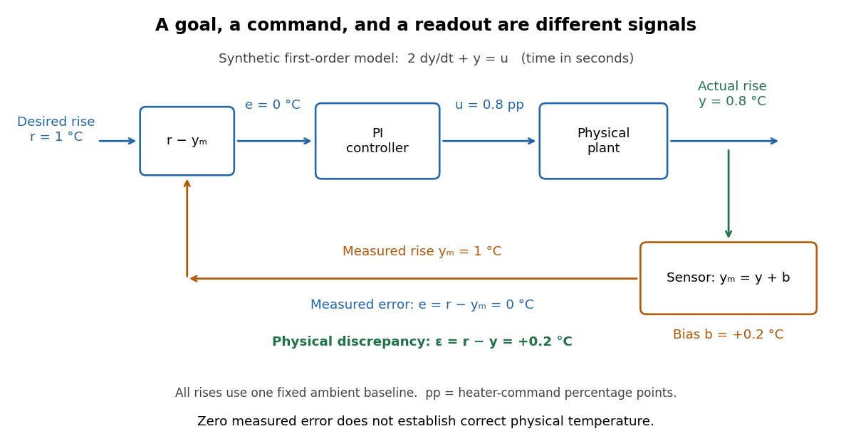
The tracking error used by the controller is the signed differencebetween the reference signal and the measured output. A positive tracking error means the readout is below the desired value; a negative tracking error means it is above. With exact measurement $y_m=y$, $r=1$ and $y=1.1$ give $e=-0.1$. For a positive-response controlled plant, positive feedback gain in proportional control $u=k_{p}e$ then reduces the plant output. The sign of the controller must also account for the sign of the controlled plant's response: a positive command that reduces the plant output requires a different sign choice. Kantor uses the opposite tracking error convention, $PV-SP$, together with a minus sign in his controller; translating both signs gives the convention here. ^[ref]

Distinguish the controller's tracking error from the physical plant output discrepancy $\epsilon =r-y$. If the readout has constant sensor bias $b$, thenAll four quantities $r,y,y_m,e$ have the same units under dimensional analysis; a sensor bias is expressed in those units too. A readout that is too high by $0.2{}^{\circ }\mathrm{C}$ can make $e=0$ when the physical temperature is $0.2{}^{\circ }\mathrm{C}$ below the goal. Integral action integrates the tracking error it receives; it cannot infer this missing calibration information from that tracking error alone. Thermometer calibration against an independent reference addresses a different problem from tuning a feedback gain.

A motivating apparatus/model comparison is Park, Martin, Kelly and Hedengren's temperature-control laboratory: two TIP31C heaters with attached TMP36GZ sensors and heat sinks, an Arduino, a power supply, and a USB-connected computer. The readout converts sensor voltage to temperature; software records that measured output while specifying heater commands from $0$ to $100\%$. For the single-heater test, one command changes in steps and the other heater stays off. Parameters are fitted to one run, then a different command sequence tests predictions without feeding measured temperatures into the simulation. The authors observe that their richer thermal model predicts the response better than the approximation with a single time constant and a delayed control input, especially after command changes. The real sensor has its own thermal lag. They also repeat the same command profile at different ambient temperatures and find changes in the response, motivating ambient-condition reporting. This experiment measures a command-to-readout response, not independently the exact heater temperature or delivered power. ^[ref]

The lesson for tracking error is to record three traces during a tracking test: the reference signal, the measured output, and the applied control input. Their first difference is the tracking error; a model prediction minus a readout is instead a model discrepancy. In a proposed comparison of proportional control and proportional-integral control, keep the initial temperature, ambient conditions, heater limits, and target changes fixed; run the second heater separately as a known control disturbance. Independent thermometer calibration is needed to assess physical accuracy. These are suggested controls, not additional experiments claimed for the paper. A sensor's lag, measurement noise, actuator saturation, and changed ambient conditions can all invalidate conclusions drawn from the ideal first-order model.