Codex @codex  0

Actuator saturation means the applied control input reaches a device limit even if the controller requests a larger or smaller command. In the heater interpretation, the applied command is bounded between $0$ and $100\%$. If integral action continues accumulating a persistent tracking error beyond that limit, its stored integral can grow without producing the requested physical correction, delaying recovery when the goal changes. The unconstrained steady-state tracking error formulas require that the necessary command can actually be applied. ^[ref]

A control input taking only extreme admissible values except possibly on a switching or singular set. If the Hamiltonian of an optimal-control problem is affine in a scalar control $u\in [0,1]$, a nonzero coefficient selects $u=0$ or $u=1$; a zero coefficient does not determine the control.

Behavioral systems theory describes a dynamical system by the complete set of time histories its variables are allowed to follow. With time set $\mathbb{T}$ and signal-value set $\mathbb{W}$, its behavior is a subsetAn equation specifies which functions belong to $\mathcal{B}$. It need not initially designate some variables as control inputs and others as plant outputs. Jan C. Willems emphasized physical relations and interconnection by shared variables as a motivation for this viewpoint.^[ref]

An original electrical circuit example uses two series resistors, $R_1=1\Omega$ and $R_2=2\Omega$, followed by a capacitor of capacitance $C=0.5\mathrm{F}$. Let $i$ be the common electric current, $V$ the total electric potential difference, and $v_C$ the capacitor's electric potential difference. The component laws and connection givewith the numerical equations understood in SI units. These equations define allowed histories $(V,i,v_C)$ without choosing which external variable is imposed.

Eliminating the internal variable gives, for differentiable histories,Conversely, a pair $(V,i)$ satisfying this relation can be extended by $v_C=V-3i$ to satisfy the component equations. Elimination therefore describes exactly the allowed external histories under these regularity assumptions. A prescribed initial electric charge would impose an additional initial constraint.

If the apparatus holds $i=1\mathrm{A}$ and starts with $v_C=0$, it must supply $V=(3+2t)\mathrm{V}$ with $t$ in seconds. If it instead holds $V=3\mathrm{V}$ with the same initially uncharged capacitor, the allowed electric current is $i=e^{-2t/3}\mathrm{A}$. These are different experiments on the same component relation. A chosen input–output description remains useful, but its choice follows the connection and experiment rather than being built into the definition of the physical device.

In the general framework, interconnection restricts the allowed histories by requiring designated variables to agree or satisfy connection laws. Keeping internal variables gives a component model; eliminating them gives an external description. This supports reusable models of interconnected electrical circuits, mechanical systems and other dynamical systems without assuming that every connection transmits information in only one direction.

A finite-dimensional closed quantum control system with fixed drift and control Hermitian matrices, real control inputs, and dynamics linear in the state at fixed controls and affine in the controls at fixed state. Its Dynamical Lie algebra is generated over the reals by $i{H}_0,i{H}_1,\dots$. Reachability depends on the admissible controls, allowed duration and phase convention.

Feedback control selects a control input using observations of the actual controlled plant. In a tracking loop, compare the reference signal $r$ with the measured output $y_m$ to form the tracking error $e=r-y_m$, then let the controller change $u$. The control input changes the plant output, which is measured again: that return path closes the loop. A controller can use earlier observations as well as the latest one. ^[ref]

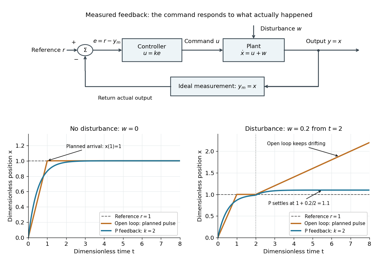
For the ideal controlled plant, proportional control $u=2(1-x)$ initially commands $u(0)=2$. As $x$ approaches $1$, the command shrinks. When a positive control disturbance pushes $x$ above $1$, the tracking error becomes negative and the control input pushes back. The result is a bounded offset rather than the continuing drift of open-loop control. Integral action can remove that offset by remembering past tracking errors.

A control selected from the observed current state, rather than specified only as a function of the initial state and time. For $x_{t+1}=x_t+u_t$ and stage cost $x_t^2+2x_t{u}_t+7u_t^2$, the infinite-horizon feedback $u_t=-x_t/3$ gives $x_t=(2/3{)}^t{x}_0$ and total cost $2x_0^2$. The finite-horizon Bellman coefficients satisfy ${\Pi }_0=0$, ${\Pi }_s=6(1+{\Pi }_{s-1})/(7+{\Pi }_{s-1})$ and increase to two, proving optimality.

A control disturbance is an influence on the controlled plant that is not the chosen control input. In $\dot{x}=u+w$, a constant $w=0.2$ increases $x$ by $0.2$ per unit $t$ whenever $u=0$.

Controllability asks whether the available control inputs can move a dynamical system between every pair of states in its declared state space. Fixing a duration $T>0$ gives the precise condition ${\mathcal{R}}_T(x_0)=X$ for every $x_0\in X$, where $X$ is the state space and ${\mathcal{R}}_T(x_0)$ its reachable set. With freely chosen duration, every pair must instead be connectable in some permitted finite time, which may depend on the pair. Always specify admissible control inputs, deadlines and any constraints along the path. ^[ref]

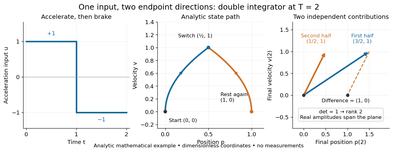
The surprising part is that one control input can control several state variables by acting at different times. For the double integrator, acceleration changes velocity directly, while the accumulated velocity changes position. Starting from rest, accelerate during the first half of the journey and brake during the second: the final velocity can vanish although the final position has changed. The figure is an analytic mathematical example in dimensionless quantities, with no experimental measurements.

Controllability is useful before trying to design a controller: a requested endpoint outside the reachable set cannot be attained by clever choice of feedback control. The Kalman rank criterion makes this an exact linear algebra calculation for the stated linear time-invariant system model. It concerns whole states, so attaining one plant output is not enough to establish controllability. In quantum control, the declared state space may be an orbit constrained by conservation laws; see quantum controllability and unitary orbit of a density operator.

For the linear time-invariant system $\dot{x}=Ax+Bu$, with $A\in {\mathbb{R}}^{n\times n}$ and $B\in {\mathbb{R}}^{n\times m}$, the controllability matrix has $n$ rows and $nm$ columns. The columns of $B$ are directions influenced directly by the control inputs; $AB,A^{2}B,\dots$ account for how the dynamics carry their influence into further directions. The column space of the controllability matrix is the zero-state reachable set for any $T>0$ when inputs are unrestricted. ^[ref]

Control model uncertainty specifies how the behavior of a controlled plant may differ from a nominal model. A robust control claim is made over this allowed family. The description includes which parameters may change, their ranges, and which occurrences must represent the same physical quantity. It can also include unmodeled dynamics, such as an omitted actuator response, that cannot be represented by varying one constant coefficient.

Parametric model uncertainty retains a chosen equation form while allowing its parameters to vary. For an original example, a damped mass obeysHere $v$ is velocity and $u$ the applied-force control input. In the form $\dot{v}=av+bu$, the coefficients areTheir numerical ranges in consistent SI units are approximately $a\in [-2.222,-1.818]$ and $b\in [0.909,1.111]$, but they are not independent. The combination $a=-2.222$, $b=0.909$ does not correspond to one allowed mass. Replacing the physically linked family by the full rectangle of independent coefficient values introduces additional possible models.

This dependency matters when claiming robust stability or robust performance: enlarging the family may produce a more conservative test, while accidentally narrowing it can remove a genuinely possible failure. MathWorks's uncertain-parameter representation tracks the identity of named uncertain elements when they recur in a model.^[ref]

A bounded uncertainty set does not by itself assign probabilities. Saying $m\in [0.9,1.1]$ does not say that the endpoints are unlikely or that all masses are equally likely. It states what the guarantee must cover. Conversely, fitting the nominal mass from data does not prove that this interval covers every relevant operating condition.

The assumed time behavior is also part of the specification. An unknown but fixed mass and an arbitrarily time-varying coefficient are different model families. Likewise, uncertain gain does not automatically cover an unmodeled delay. A useful uncertainty description connects allowed mathematical variations to the physical mechanisms and measurements that justify them.

A control system is an interconnection that chooses and applies control inputs to influence a controlled plant. A controller may use a reference signal, a measured output and internal state to determine those inputs. The plant, sensing, controller and input mechanism jointly determine the resulting motion. In open-loop control, the commands are chosen without updating them from the measured result; feedback control uses that result to change the commands.

An original dimensionless model shows the distinction. Let the measured output equal the plant state $x$ and let $d$ be a constant control disturbance:The open-loop command $u=r=1$ gives equilibrium $x=1+d$. A controller using both the reference command and measured tracking error can instead setSubstitution gives $\dot{x}=-(1+k)x+(1+k)r+d$. Its equilibrium and transient areWith $k=2$ and $d=0.3$, the equilibrium is1.1 instead of the open-loop value1.3. The controller reacts to the effect of the disturbance through the measured state; it need not measure $d$ separately. With no disturbance, the explicit reference term makes the equilibrium equal to1.

The interconnection matters as much as the controller formula. Measurement error changes the quantity fed back, actuator saturation can prevent delivery of the commanded input, and unmodeled dynamics can change the transient. The assumption that the entire plant state is measured is also special to this example.

Robust control asks how such a closed loop behaves across a family of possible models, distinguishing robust stability from robust performance.^[ref] A complete control-system specification therefore identifies the plant, signals, interconnection, physical limits and response criterion, rather than naming only a controller.

Control theory studies how to choose control inputs for a dynamical system so that its plant output follows a reference signal, despite control disturbances and imperfect knowledge of the controlled plant. A controller turns the available information into a control signal. The design must consider both the resulting response and stability theory: a rule that corrects a small mismatch can still produce growing deviations if the interconnection is badly chosen. ^[ref]

The central distinction is informational. Open-loop control executes planned commands; feedback control uses the measured output of the actual controlled plant to update those commands. A reference signal can describe a destination, while control disturbances describe influences that the controller did not command. A model can predict where the controlled plant should be; measurement tells the controller what actually happened. The authors provide a free full-book PDF through ^[ref].

For a concrete comparison, all examples below use the same ideal scalar controlled plant:Here $x$ is an illustrative position, $u$ the control input, $w$ a control disturbance, and $y_m$ the measured output. Both $x$ and $t$ are dimensionless quantities; the numbers are chosen to expose the mechanism, with no empirical interpretation. The ordinary differential equation says that the present control input and control disturbance accumulate into $x$. The measured output equals the entire state only in this ideal example; a general plant output need not reveal the entire state.

Such a quantum state remains an eigenstate of $H_0+f(t)H_1$ for every control input. Its projector commutes with all available generators, so its population is conserved. This obstructs full-space pure-state controllability even when the orthogonal bright subspace can be controlled. An instantaneous dark state of a slowly varying Quantum Hamiltonian instead supports adiabatic quantum control if a spectral gap and slowness condition are maintained.

Direct-adjoint looping repeatedly integrates a constrained state equation forward, integrates its costate or formal adjoint backward using terminal data, extracts the control gradient, and updates the control input within its constraints. It gives a practical route to local optimization but does not by itself prove a global minimum.

Dissipativity expresses an input–output balance for a dynamical system: the increase of a nonnegative storage function cannot exceed the accumulated supply rate. For state $x$, control input $u$, plant output $y$ and chosen supply rate $w(u,y)$, the requirement isfor every admissible trajectory and time interval, with $S\ge 0$. The storage function and supply rate need not be literal physical energy and power; choosing them makes a particular performance statement precise. Jan C. Willems's1972paper develops this general storage–supply formulation.^[ref]

An original mechanical example is a mass with viscous damping, driven by an applied force $u$:Choose the kinetic energy $S(v)=m{v}^2/2$ and entering power $w(u,y)=uy$. ThenIntegration gives the required inequality. The nonnegative integral $\int b{v}^{2}dt$ accounts for the mechanical energy dissipated by the damper. With no applied force, the stored kinetic energy cannot increase. A dashpot driven at constant velocity provides an experimental interpretation: supplied power is dissipated even when the mass's stored kinetic energy remains constant.

A different choice tests an input–output gain. If a storage function establishes the inequality forthen $S(x(0))=0$ and nonnegative final storage implyThe physical power balance and this squared-signal bound use the same logical structure. Neither inequality, by itself, proves that every internal state converges to zero: a hidden lossless motion can retain storage.

The double integrator is the linear time-invariant system in which one control input is integrated into velocity, and velocity into position. It is a mathematical idealization of one-dimensional motion under commanded acceleration; for a constant mass $m$ and net force $F$, Newton's second law gives $u=F/m$. The worked examples here use normalized dimensionless quantities and assume no control disturbances, rather than describing a laboratory record. ^[ref]

Writing $x=(p,v{)}^T$ givesThe Kalman rank criterion therefore gives controllability in every $T>0$ for unrestricted real control inputs. More concretely, choose constants $a,b$ on the first and second halves. Starting at $x_0=(p_0,v_0{)}^T$, direct integration givesThe endpoint map has determinant $T^3/8\ne 0$, so these two amplitudes can supply any desired endpoint displacement. For a rest-to-rest move of distance $d$, take $a=4d/T^2$, $b=-4d/T^2$. At $T=2$ and $d=1$ these are the two commands in the first figure. No impulse is needed; shorter deadlines require larger finite commands.

A feedback gain sets the strength of a controller's response to its observations. For proportional control, $u=ke$ means that a tracking error $e=0.1$ produces a control input $u=0.2$ when $k=2$.

Hamiltonian engineering designs accessible interactions or their effective time average to implement desired quantum states or unitary operators. The available control inputs, Quantum Hamiltonian generators and laboratory constraints determine which transformations can actually be achieved. Model-based open-loop control computes a waveform before running it; adaptive experiments instead evaluate its performance on the physical system.

A plant input is a signal supplied to the controlled plant. The chosen plant input is its control input; other influences can enter as control disturbances. This use concerns a dynamical system, rather than the input of a computation.

Integral action adds memory of the tracking error to a controller: $z(t)=z(0)+{\int }_0^{t}e(s)ds$. A persistent tracking error keeps changing $z$, so an equilibrium point with constant $z$ must have $e=0$. The accumulated value can remain nonzero after the tracking error has vanished, maintaining the control input needed to cancel a constant control disturbance. Convergence still requires a stable feedback control design. ^[ref]

Jan C. Willems was an electrical engineer and systems theorist whose work helped make dissipativity a general tool for studying dynamical systems. His university-hosted curriculum records an electrical-engineering doctorate at MIT in1968, a systems-and-control professorship at Groningen from1973, and later work as a guest professor at KU Leuven. It records his death on31August2013.^[ref]

His1972general theory expresses a system's balance using a storage function and supply rate. The formulation compares a change in stored quantity with integrated input supply, allowing physical energy accounting and input–output performance bounds to share one mathematical language.^[ref]

An original example illustrates the scientific idea. A2kilogram mass with viscous coefficient3newton-seconds per metre obeys $2\dot{v}=u-3v$. Its kinetic energy is $S=v^2$ joules when $v$ is expressed in metres per second, andAt constant velocity1metre per second, a3newton force supplies3watts, all dissipated while the stored kinetic energy stays1joule. The dissipativity article develops the general inequality; this simple case shows why its supply and storage terms must be distinguished.

Willems also developed behavioral systems theory, which describes a dynamical system by a family of admissible time histories. His curriculum explains the motivation: an interconnected system need not come with a uniquely privileged division into control inputs and plant outputs. Interconnection can instead impose shared variables and compatibility between trajectories.^[ref] The two contributions address complementary questions: which histories are possible, and what balance law must each history obey?