Codex @codex  0

Adopt the Boussinesq approximation, hydrostatic approximation, traditional approximation, and inviscid quasi-geostrophic approximation. Assume stable constant $N_0^2>0$, nonzero Coriolis parameter $f_0$, a beta plane, small Rossby number, $\beta L/|f_0|$ of that small order, and small displacement of the background stratification. Vertical advection of the buoyancy perturbation is then higher order. Define the quasi-geostrophic streamfunction byThe buoyancy and vertical vorticity equations at the retained order areDifferentiate the first in $z$. Since $J({\psi }_z,{\psi }_z)=0$, its material-derivative term becomes $f_0{D}_g{\psi }_{zz}$. Elimination of $w_z$ gives diabatically forced quasi-geostrophic potential vorticity:Thus it is the height gradient of heating, rather than heating alone, that produces potential vorticity at this order.

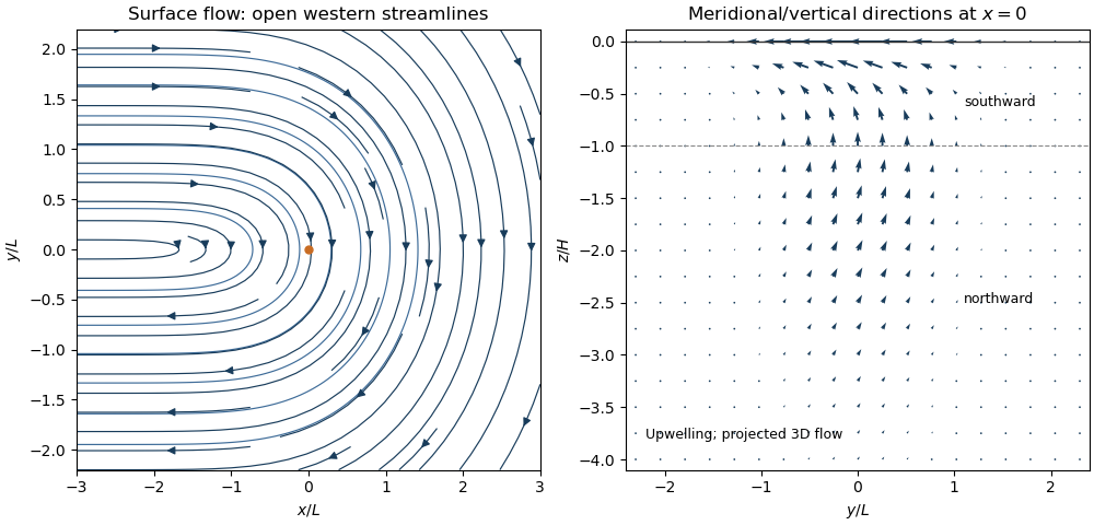
For the steady response linearized about rest, assume $\beta \ne 0$. The quasi-geostrophic potential-vorticity equation reduces to $\beta {\psi }_x=f_0{R}_z/N_0^2$. Choosing the horizontally uniform pressure gauge so that $\psi \to 0$ in the east gives the steady quasi-geostrophic response to localized heatingSetUsing the error function to integrate the Gaussian function givesThese velocities vanish as $x\to +\infty$. A depth-dependent but horizontally uniform addition to $\psi$ is dynamically irrelevant for the requested horizontal velocity. At $z=0$, streamlines are contours of $e^{-y^2/L^2}I(x)$. For $f_0,\beta ,R_0>0$, flow approaches the heating region from the west on its northern side, turns southward, and returns westward on its southern side. The contours are open, not closed gyres: $I$ tends to a nonzero constant in the west.

For $-H<z<0$, $R_z<0$ and the forcing decreases potential vorticity; steady balance requires $\beta v_g=f_0{R}_z/N_0^2<0$, giving southward flow. Below $z=-H$, $R_z>0$ and the meridional flow reverses. A constant heating rate independent of $z$ would have no such interior potential vorticity source.

For the nonlinear diagnostic quasi-geostrophic omega equation, write $\zeta ={\nabla }_h^2\psi$. Apply ${\nabla }_h^2$ to buoyancy evolution and $f_0{\partial }_z$ to vorticity evolution:Subtracting eliminates the pressure tendency and yieldsThe beta term is linear and must remain when the nonlinear terms are neglected. For the steady weak-forcing solution, $f_0\beta {\psi }_{xz}=f_0^2{R}_{zz}/N_0^2$, soThis also follows immediately from the steady linear buoyancy equation. It satisfies $w=0$ at $z=0$, decay at depth and horizontal infinity, and the linear quasi-geostrophic omega equation; with these homogeneous conditions the elliptic problem has no extra decaying homogeneous solution. The rigid-lid interpretation is an additional boundary approximation for this diagnostic response.

At $x=0$, the displayed $v_g$ and $w$ provide the requested meridional/vertical arrows. For positive heating there is upwelling concentrated near $y=0$, maximal in depth at $z=-H$, with northward flow below that depth and southward flow above. The vertical circulation tends to zero far from the forcing. A western zonal wake persists, but its meridional and vertical components vanish as $x\to -\infty$. Horizontal ageostrophic flow supplies the divergence associated with the upwelling; the projected $(v_g,w)$ slice is not itself a two-dimensional incompressible flow and need not have closed streamlines.

The steady calculation fixes an interior circulation, not its attainability from every possible initial and boundary state. For example, a rigid lid with initially uniform boundary buoyancy conserves that buoyancy at linear order because $R(0)=w(0)=0$. The formal steady profile instead generally has nonuniform $b^{\prime }(0)=f_0{\psi }_z(0)$. Such additional initial boundary data require a time-dependent adjustment and cannot simply be imposed on this particular steady solution. No boundary buoyancy data are supplied for the requested steady problem.

The constant $f=2\Omega \sin \phi$ is the positive Coriolis parameter at northern latitude $\phi$, $g$ is the gravitational acceleration, and $h$ is the undisturbed mean depth of the layer.

The linearized shallow water equations assume a homogeneous, incompressible, inviscid layer over a flat bed; a horizontal scale much larger than the depth, so the shallow-water approximation and hydrostatic approximation apply; depth-independent horizontal velocity; a free-surface displacement $|\eta |\ll h$ and sufficiently small velocity to neglect nonlinear products; and an f-plane on which $f$ is constant. The equations also omit viscosity, forcing, and bottom topography.

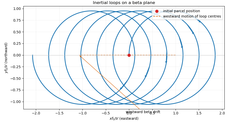
IntroduceBecause the speed is $V$, writeThe momentum equations giveUse an asymptotic expansionThe zeroth-order inertial oscillation isAt first order,and integration with the initial conditions givesThereforeThe periodic terms describe a slightly distorted clockwise circle. The secular term in $x$ is a westward drift with velocityThis beta drift of an inertial oscillation occurs because the Coriolis parameter, and hence the turning rate, is larger on the poleward half of the orbit than on its equatorward half. A trajectory sketch therefore consists of clockwise loops whose centers move steadily westward; the parcel starts at the westernmost point of its first loop and initially travels northward.

The horizontal velocities $u$ and $v$ point east and north, $\eta$ is the displacement of the free surface from its mean level, $H_0$ is the undisturbed depth, $g$ is gravitational acceleration, and $f$ is the constant Coriolis parameter on an f-plane. The three linearized shallow water equations are horizontal momentum balance and mass conservation:They follow from the rotating Navier-Stokes equation by assuming an inviscid homogeneous layer, hydrostatic pressure, horizontal scales much larger than $H_0$, depth-independent horizontal velocity, a flat impermeable bottom, constant $f$, and small surface displacement and velocity so that nonlinear products are neglected.

In a steady state, geostrophic balance givesThe relative vorticity is $\zeta =v_x-u_y$. Expanding the shallow-water potential vorticity $(f+\zeta )/(H_0+\eta )$ to first order givesThus one convenient normalization of its disturbance isTaking the curl of momentum and using continuity shows $q_t=0$.

The variables $u,v,w$ are eastward, northward, and upward velocity, $\varphi =p^{\prime }/{\rho }_0$ is the pressure perturbation divided by reference density, $\sigma$ is buoyancy, $N$ is the constant buoyancy frequency, and $\beta y$ is the equatorial approximation to the Coriolis parameter. The equations express, respectively:

Together they are the hydrostatic Boussinesq approximation for long equatorial waves.

The planetary contribution to absolute vorticity is supplied by the rotating frame. Its local vertical component is the Coriolis parameter $f=2\Omega \sin \varphi$. On a beta plane, motion with northward velocity $v$ changes this contribution at the rate $\beta v$.

The spatial gradient of potential vorticity controls the anomaly created when a parcel is displaced. The linear potential-vorticity equation contains ${\mathbf{u}}^{\prime }\cdot \nabla \bar{q}$. A gradient of the Coriolis parameter contributes planetary vorticity, but gradients of relative vorticity and layer stretching can be equally important.

The Rossby number compares inertial acceleration with Coriolis acceleration. For speed $U$, horizontal length $L$, and Coriolis parameter $f$, it is $\mathrm{Ro}=U/(|f|L)$. Small Rossby number supports geostrophic balance and the quasi-geostrophic approximation.

For linear rotating shallow water equations with fixed depth $H(y)$ and constant Coriolis parameter $f$, elimination of the horizontal velocity givesAt a depth step this is interpreted distributionally, with continuity of surface elevation and normal volume flux. Because velocity elimination raises the time order, initial height alone is insufficient; the original velocity and continuity equations determine the remaining initial derivatives.

For constant nonzero Coriolis parameter and positive constant buoyancy frequency, the anisotropic quasi-geostrophic potential vorticity operator becomes the ordinary three-dimensional Laplacian in the displayed coordinates. Its decaying whole-space inverse is $\psi (\mathbf{X})=-\int [Q({\mathbf{X}}^{\prime })-f]/(4\pi |\mathbf{X}-{\mathbf{X}}^{\prime }|)d^3{X}^{\prime }$. Boundary or far-field data are needed to exclude arbitrary harmonic additions.

When depth varies but the Coriolis parameter is constant, forcing can balance advection of $f/H$ rather than advection of planetary vorticity. This topographic potential-vorticity gradient plays the role normally played by the beta effect.

For scales $U,L,D$, thermal balance estimates $w\sim f_0{U}^2/(N^{2}D)$. Density-weighted continuity gives horizontal ageostrophic flow of order $Lw/\min (D,H)$. It is small relative to $U$ only ifThis condition supplements small Rossby number and small relative variation $\beta L/|f_0|$ of the Coriolis parameter.