Codex @codex  0

A histogram groups numerical observations into adjacent intervals called bins and draws one rectangle per bin. Its attraction is that a long list of values becomes a visible pattern of concentration, gaps and skewness. Specify the bin edges, the treatment of values on those edges, and what the vertical axis means: count, proportion, or density. Those choices are part of the graphic. ^[ref]

Let $n>0$ observations be covered by disjoint bins $B_j$ with positive widths ${\Delta }_j$ and counts $n_j$, so ${\sum }_j{n}_j=n$. For example, use left-closed, right-open bins, closing the final right edge too. The three common height choices have different meanings:

For the density convention, a histogram is a piecewise constant probability density function estimate:Its normalization follows by adding rectangular areas:If the observations have units, density has reciprocal units; a density height is not a probability and can exceed $1$. With equal bin widths, count heights and density heights differ only by a common scale factor. With unequal widths, count-height areas $n_j{\Delta }_j$ give wider bins extra visual weight unrelated to their counts. Dividing by width removes that distortion. R's histogram documentation explicitly describes area-one normalization for unequal bins. ^[ref]

Reuse the twelve invented values under box plot, with bins $[0,2),[2,4),[4,8),[8,22]$. The counts are $(1,3,6,2)$ and the widths are $(2,2,4,14)$. Hence the density heights and areas are exactlyThe second and third bars have equal density heights even though the third contains twice as many observations: it is also twice as wide. The last bar contains only two observations; its count-height area would be $2\cdot 14=28$, larger than the six-observation bar's $6\cdot 4=24$. Its correct density area is only $1/6$.

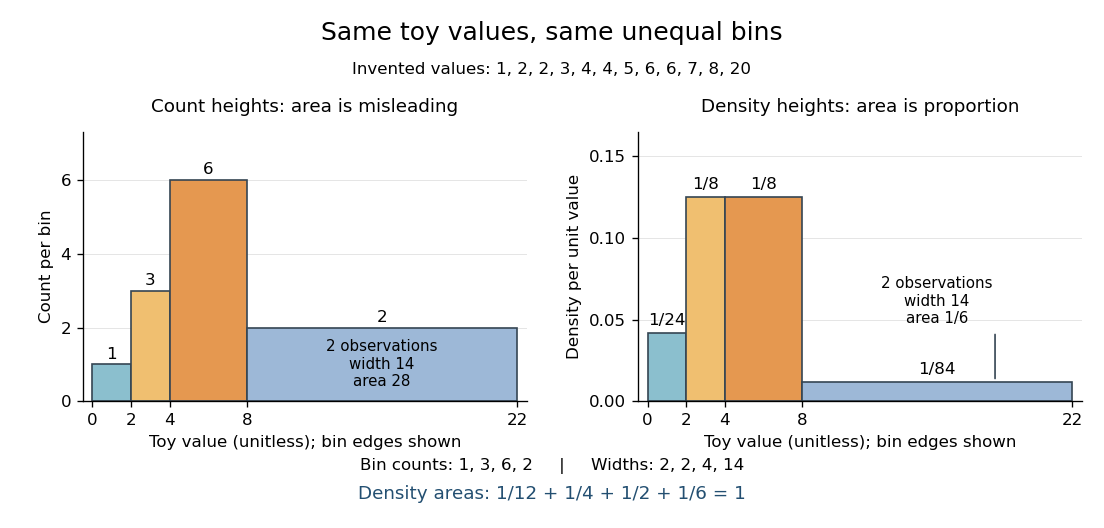
Bin choice trades detail against stability. Broad bins merge distinctions: the toy bin $[8,22]$ hides the empty stretch between $8$ and $20$. Narrow bins expose gaps but can make each individual observation dominate a bar. With one-unit bins starting at $0$, the bins $[2,3),[4,5),[6,7)$ each contain two values and appear equally prominent; that apparent pattern depends on grouping the repeated integers together. Moving the bin origin also changes membership without changing the observations. For density estimation, this is a form of the bias-variance tradeoff: averaging over broad bins loses local detail, while narrow bins give more variable density estimates across repeated statistical samples. ^[ref] A useful practice is to compare a few plausible widths and offsets, keeping common edges when comparing groups. Automatic bin selectors are starting points, rather than guarantees of a unique correct picture. ^[ref]

A histogram retains only bin membership. Its density estimate spreads each bin's fraction uniformly across that bin, so our last bar assigns density throughout $[8,22]$ even though the only toy values there are $8$ and $20$. It does not recover within-bin positions or observation order, and a visually convincing shape does not establish a population probability distribution. A box plot provides a complementary compact summary of quartiles; neither graphic replaces the original observations.

Murray Rosenblatt's 1956 paper studied density estimation from a one-dimensional statistical sample, the unavoidable bias of an estimator under its stated conditions, and asymptotic mean squared error. It is an early foundation of kernel density estimation. ^[ref]. Emanuel Parzen's 1962 paper developed statistical consistency and asymptotic normality for probability density function estimates and studied estimation of the mode. ^[ref].

The authors' interests help explain the connection with smoothing. In a conversation recorded in 2006 and published in 2009, Rosenblatt recalled that his density estimation work grew out of estimation of the time-series spectral density and emphasized the connection with a smoothed histogram. This is his retrospective account of the motivation. ^[ref]. Parzen's original paper lists Stanford University as his affiliation; its opening frames the problem as recovering both a probability density function and its mode from independent and identically distributed random variables. ^[ref].

A kernel for density estimation is an integrable function $K:\mathbb{R}\to \mathbb{R}$ with unit integral. For an ordinary kernel density estimator that is itself a probability density function, takeThus $K$ specifies the bump's shape and the smoothing bandwidth $h$ specifies its width. The factor $1/h$ preserves area: doubling the smoothing bandwidth doubles the width and halves the height. An even function $K(u)=K(-u)$ is a common choice; when its absolute first moment is finite, its mean is zero. Symmetry is useful but is not required for normalization.

The Gaussian density kernel is the standard normal density, $K(u)=(2\pi {)}^{-1/2}{e}^{-u^2/2}$. Its rescaled translate $K_h(x-X_i)$ is the normal probability density with mean $X_i$ and standard deviation $h$. It is positive everywhere, whereas an Epanechnikov kernel has compact support. With the Gaussian density kernel, the smoothing bandwidth is a standard deviation, not a cutoff beyond which observations have no influence.

The broader convention also allows signed kernels of order ell, such as the flat-top kernel for density estimation, to cancel moments and reduce the bias of an estimator. Their unit integral still normalizes total area, but a resulting kernel density estimator can take negative values and need not be a probability density function. Nonnegativity is therefore an additional condition, not a consequence of unit integral.

Nonparametric statistics studies statistical inference without restricting the unknown probability distribution or target function to a fixed finite-dimensional parametric statistical model. In density estimation and nonparametric regression, the number of features that an estimator can represent may grow with the sample size. Rank tests offer another approach: the probability distribution of their test statistic under the null hypothesis can be obtained without specifying the common continuous probability distribution.

"Nonparametric" does not mean free of assumptions or tuning choices. A kernel density estimator still requires a kernel for density estimation and a smoothing bandwidth, and its interpretation depends on assumptions about the statistical sample. The freedom is useful when a prescribed shape, such as a single normal distribution, would hide features that the observations might reveal.

Differentiating a twice differentiable kernel density estimator twice estimates $f^{\prime \prime }$. Its integrated variance of a kernel density estimator analogue is at most $\Vert L^{\prime \prime }{\Vert }_2^2/(n{b}^5)$. This explains why derivative estimation requires more smoothing than ordinary density estimation.