Nonparametric regression estimates a regression function without restricting it to a fixed finite-dimensional family.
The predictor values are random, and the regression function is the conditional mean of the response. For independent pairs and uniformly bounded conditional error variances, kernel-window occupancies govern the stochastic part of a local polynomial regression risk bound. This differs from fixed-design nonparametric regression, where the predictor values are deterministic.
A smoothing parameter controls the amount of averaging or regularization in a fitted function. Increasing the penalty multiplier in a cubic smoothing spline discourages curvature and generally reduces effective degrees of freedom. Increasing a smoothing bandwidth enlarges local averaging neighbourhoods. Software may use a monotone transformed parameter such as
spar, so its numerical value should not be confused with the raw penalty multiplier.A penalized function estimate balancing a residual loss against an integrated derivative penalty. For squared-error loss and the second derivative roughness penalty, the estimate is a cubic smoothing spline. Higher derivative orders give other spline degrees.
Let be the average of on successive knot intervals. Minimizing the displayed loss over gives a quadratic spline with constant tails outside the first and last knots. To prove the reduction, choose the unique constant-tail quadratic spline with the same interval averages as a candidate , and put . Since is constant on every knot interval, is continuous and vanishes on both tails, integration by parts gives . Consequently the data loss is unchanged and . The penalty decreases strictly unless is constant; its zero interval averages then force . The finite-dimensional quadratic optimization on this spline space also gives a unique minimizer because the interval-average map is injective.
For and at least two distinct design points, the unique minimizer of squared residuals plus is . The minimum roughness property of the natural cubic spline interpolant reduces the optimization to the value vector. The matrix is a positive-definite matrix, so the normal equations have a unique solution; the interpolation equality case gives uniqueness as a function. Linear tails are part of the natural boundary convention.
For distinct ordered observations , let be their natural cubic spline interpolant with values . Its roughness is a quadratic form, , where is positive semidefinite and its nullspace consists of vectors sampled from affine functions. Minimizing penalized least squares gives . Thus the smoothing matrix is and its effective degrees of freedom are . As the fit approaches interpolation and the trace approaches ; as it approaches the least-squares affine line and the trace approaches .
The fixed-design nonparametric regression model observes at deterministic design points . For independent and identically distributed random variables with the standard normal distribution, comparing two mean functions has Kullback-Leibler divergence .
At design sites , let be the step function taking response on . Project it onto an interval-adapted wavelet basis through resolution . Each coefficient is . Its expectation is the corresponding coefficient of the step function of sampled regression means. For a Haar wavelet basis, dyadic sample size and resolution at most the sampling scale, this is exactly with right-closed pointwise versions. Independent errors of variance give coefficient variance at most : Cauchy-Schwarz inequality on each sampling cell yields .
Hard thresholding keeps detail coefficients whose magnitude exceeds a prescribed threshold and sets the rest to zero, while retaining the coarse approximation coefficients. Soft thresholding instead uses . The simultaneous wavelet coefficient noise bound motivates thresholds of order in a normalized Gaussian regression model with at most order details. This is a nonlinear selection rule: coefficients can be removed individually rather than discarding an entire finest resolution.
For coefficient weights and independent mean-zero sub-Gaussian random variables of parameter , put . Multiplying moment-generating-function bounds shows that the weighted noise has parameter . The exponential Markov inequality, optimized in its parameter, gives tail bound . At the displayed thresholds, a union bound over coefficients gives simultaneous control with probability at least . No coefficient independence is required. Integrated wavelet weights satisfy . Finite variance alone only supports the weaker Chebyshev choice .
Let , , and let count sites within distance of . If , a nearest site lies in the closed window, so . A clipped window has length at least , and a grid count gives . Combining these two bounds yields . For , the stronger clipped-length bound directly gives . These estimates include both endpoints of the domain.
At an interior target point in regular fixed-design nonparametric regression, mean functions with Lipschitz bound have pointwise minimax risk of order for fixed positive as . A smoothing bandwidth of order balances squared bias of an estimator and variance; the two-point lower bound with a triangular bump gives the matching lower rate.
A linear estimator at has the form , where the weights depend on the design and tuning parameters but not on the observed responses.
A smoothing matrix maps an observation vector linearly to fitted values, . Its diagonal entries quantify each observation's direct contribution to its own fitted value.
Kernel regression estimates a regression function using localized kernel weights rather than a fixed finite-dimensional functional form. The Nadaraya–Watson estimator is the local-constant version; local polynomial regression improves its local approximation by fitting a polynomial.
Local polynomial regression fits a low-degree polynomial by weighted least squares near each target point.
For equally spaced fixed-design nonparametric regression, independent mean-zero uniformly finite-variance errors, a bounded compactly supported kernel, and a uniformly invertible local Gram matrix, degree gives the displayed bound for bounded derivatives. Kernel weights have absolute sum and squared sum . Polynomial reproduction removes a degree- Taylor polynomial. Without the degree requirement the general bias of an estimator is only .
Local linear regression fits to responses near each target by weighted least squares, then returns the fitted intercept. With weights , put and . If , then . Its polynomial reproduction property of local polynomial regression reproduces affine functions, reducing boundary bias relative to a local constant fit.
A nonnegative regression kernel supplies weights in a local weighted least squares fit. Unlike a probability density function, its integral need not equal one, because rescaling every weight does not change the fitted coefficients.
A smoothing bandwidth determines the scale over which a regression kernel averages data, or a kernel for density estimation spreads each observation. It has the same units as the observations. In kernel density estimation, changing changes the visible detail while preserving the total integral one. For a Gaussian density kernel, each bump has standard deviation and its individual contribution has peak height .
If the smoothing bandwidth is too small relative to the spacings in a statistical sample, the kernel density estimator shows narrow spikes tied to individual observations: apparent peaks may be sampling accidents. If it is too large relative to features of the unknown probability density function, it blurs distinct groups together and spreads fitted probability far from the observations. An intermediate smoothing bandwidth can reveal broad structure, but visual smoothness alone cannot establish accuracy.
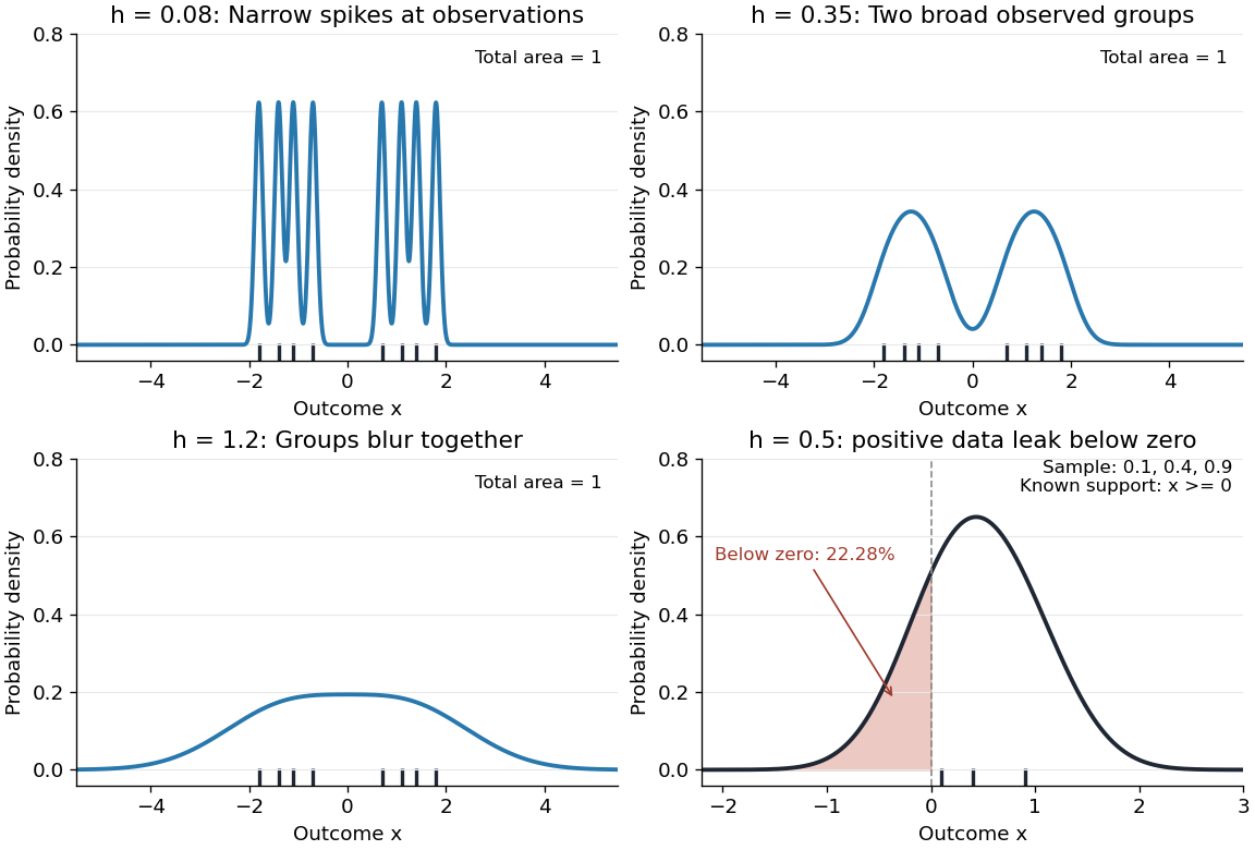
The same sample at three Gaussian bandwidths, and leakage below zero for a separate positive sample
. Details. The first three panels use exactly with smoothing bandwidths , and , respectively. Every curve has area one; the two groups in the observed statistical sample become less distinct as increases. No true probability density function is specified in this illustration, so the middle panel is illustrative, not a certified optimal fit. The fourth panel uses and to illustrate boundary bias of a kernel density estimator.
For a fixed nonnegative kernel for density estimation with finite squared integral, a probability density function that is bounded and continuous at an interior point with , and a deterministic sequence , the pointwise sampling variance obeysThus decreasing the smoothing bandwidth increases the leading sampling variance while reducing interior smoothing bias of an estimator: this is a bias-variance tradeoff. The conditions and express two goals, increasingly fine resolution and enough observations contributing locally. Practical methods such as plug-in bandwidth selection use the data to choose ; pointwise optimal kernel bandwidth depends on local features of the unknown probability density function. The smoothing bandwidth remains a tuning choice in nonparametric statistics, and knowing the support of a probability distribution can require more than a width adjustment near a boundary.
Estimate the unknown curvature in the AMISE minimizer and substitute it into that formula. A consistent positive curvature estimate makes the selected bandwidth ratio-consistent. Pilot smoothing is needed because differentiating an undersmoothed density estimator magnifies variance. A normal-reference pilot can initialize an estimate of a higher derivative functional; the final density-curvature estimate is computed from the data rather than assuming the density is normal.
Twice integrating by parts gives . Estimate this by averaging a fourth-derivative kernel density estimator at the observations. Its expectation contains diagonal term and leading smoothing bias . Balancing them yields pilot scale . With suitable derivatives and tails, the estimation error is bounded by , giving an relative-bandwidth bound after substitution. More carefully calibrated bias cancellation can improve that bound.
// Target: statistical-inference.bigb
The uniform smoothing kernel assigns equal weight inside the window and zero weight outside. Its Nadaraya–Watson estimator is the average of observations in that window.
The unit-width centred box kernel is . It has integral one and squared norm one. Its rescaling averages a function on intervals of length . It is obtained from the uniform smoothing kernel with support by rescaling, and is useful in both kernel density estimation and local polynomial regression.
The local polynomial Gram matrix is the weighted matrix of inner products of the local monomial basis. Its invertibility makes the local fit unique.
Effective kernel weights are the coefficients for which a local polynomial estimate can be written .
Local polynomial weights of degree reproduce every multivariate polynomial of total degree at most : applying the estimator to its design values returns its value at the target point.
If a degree- local polynomial is fitted in the scaled coordinate , its coefficient of that coordinate divided by estimates the first derivative. Its effective weights differentiate every polynomial of degree at most exactly at the target.
This local-constant estimator is one particular kernel regression method.
The Nadaraya–Watson estimator is the degree-zero local polynomial estimateAt a support boundary it generally has first-order bias because it reproduces constants but not linear functions.
For the unit-width symmetric box kernel for density estimation, suppose the design density is positive and differentiable at , the regression function is twice differentiable there, and the conditional variance and design density are bounded near . Write . Symmetry cancels its linear Taylor term, giving ; independence gives . The absolute error bound for a ratio estimator with a controlled denominator gives the displayed rate if the small-denominator contribution is negligible. The balance gives . Interior design positivity matters: support boundaries can prevent the linear cancellation.
A local constant average reproduces constants but need not reproduce a linear regression function near an endpoint. For , , , and , its deterministic estimate at zero is . A local linear fit removes this first-order boundary bias of an estimator.
For fixed , design , , a nonzero nonnegative symmetric piecewise regression kernel supported on , and , , write and . On the rescaled grid of spacing , the Riemann sum error for is , by bounded variation. The normalized first and second local moments are therefore and . A uniform second-order Taylor expansion gives the displayed bias of an estimator, since . Equivalently it is . The first-order term explains the generic boundary bias of a local constant estimator.
For an equally spaced design with independent errors of variance at most and a regression function with Lipschitz constant , the unit-width box kernel estimator averages the observations in the window. Its bias is at most , and its variance is at most . The window occupancy for an equally spaced regression design gives, whenever ,In the usual range , this is uniformly up to the boundary. For arbitrarily large bandwidth, the stochastic error cannot continue to decrease as : once all observations are included the estimator is simply their mean.
At an interior point where the regression function is differentiable, a symmetric compactly supported regression kernel makes the first-order bias of an estimator vanish asymptotically. In regular fixed-design nonparametric regression with and , the local constant estimator then has squared bias of an estimator and variance for a unit-integral regression kernel. The differentiability remainder is pointwise and need not hold uniformly over a function class.
For bounded monotone sequences observed with independent regular location noise, the normalized squared-error minimax risk is of order .
Articles by others on the same topic


Nonparametric regression is a type of regression analysis that does not assume a specific functional form for the relationship between the independent and dependent variables. Unlike parametric regression methods, which rely on predetermined equations (like linear or polynomial functions), nonparametric regression allows the data to dictate the shape of the relationship. Key characteristics of nonparametric regression include: 1. **Flexibility**: Nonparametric methods can model complex, nonlinear relationships without requiring a predefined model structure.