Nonparametric statistics studies statistical inference without restricting the unknown probability distribution or target function to a fixed finite-dimensional parametric statistical model. In density estimation and nonparametric regression, the number of features that an estimator can represent may grow with the sample size. Rank tests offer another approach: the probability distribution of their test statistic under the null hypothesis can be obtained without specifying the common continuous probability distribution.
"Nonparametric" does not mean free of assumptions or tuning choices. A kernel density estimator still requires a kernel for density estimation and a smoothing bandwidth, and its interpretation depends on assumptions about the statistical sample. The freedom is useful when a prescribed shape, such as a single normal distribution, would hide features that the observations might reveal.
A rank test is a hypothesis test whose statistic is a function of the ranks of observations, possibly together with fixed sample labels. Under independent observations from a common continuous probability distribution, exchangeable rank allocations give its exact null law without specifying that distribution. The Wilcoxon rank sum test is an example. Invariance under common increasing transformations follows because ranks do not change.
For independent paired observations, form differences . Assume the differences are identically distributed, continuous and symmetric about a location . Under the zero-location null hypothesis, the signs are independent fair signs conditional on their absolute values. Rank the absolute differences and add ranks with positive signs. A negative-location alternative rejects for small . Its exact conditional distribution is that of a sum of an independently selected subset of ranks, each of the subsets equally likely. Thus its mean is and its variance is . Symmetry is essential: a zero median alone does not justify this signed-rank null law. Zero differences are omitted in the usual version, and tied absolute differences receive average ranks.
The Walsh averages of a sample are for , including the diagonal pairs. If the absolute observations are distinct and nonzero, order them as . Among the pairs whose larger absolute observation is , every sum has the sign of . Hence the number of positive Walsh averages is exactly , the positive Wilcoxon signed-rank statistic. This proves equivalence of the corresponding tests; the Walsh averages themselves are generally dependent.
For a continuous sample, the statistic also equals . In each pair the sign of the sum is the sign of the observation with larger absolute value, proving the identity by counting its smaller-rank partners. Under a continuous symmetric null, the pair kernel has projection and projection variance . The U-statistic central limit theorem yields asymptotic normality of , with variance asymptotic to .
For two independent samples of sizes , rank their pooled observations and let be the sum of the ranks of the first sample. With continuous observations, the null hypothesis of a common distribution makes every allocation of ranks to that sample equally probable. A one-sided alternative that the first sample is stochastically smaller rejects for small , equivalently small . In a common-shape location model this tests a negative location difference. Without the common-shape assumption it is not simply a test of medians. The shifted statistic counts cross-sample pairs for which the first observation exceeds the second. Ties use average ranks and a conditional permutation test or a tie-adjusted normal approximation.
With and no ties, sampling ranks without replacement gives the displayed mean and variance. For observed rank sum below its mean, a continuity-corrected lower-tail statistic is . Ties of sizes replace the variance by . These formulas concern the raw rank sum; the Mann–Whitney U test statistic subtracts from both the observation and its mean.
Under the continuous common-distribution null of the Wilcoxon rank sum test, pooled labels are exchangeable. The product records every choice of ranks: choosing assigns rank to the first sample. Its indicated coefficient counts subsets of size and rank sum . Divide by and sum the lower tail for the one-sided P-value. Equivalently the counts satisfy with , allowing an exact integer computation.
For two independent continuous samples of positive sizes under a common-distribution null, each -subset of ranks is equally likely. The smallest rank sum is , attained only by . The only subset with rank sum one larger is . Hence the exact lower tail at that threshold is . This follows directly by observing that any other change increases the sum by at least two.
Independent additive noise multiplies characteristic functions: . When the noise characteristic function is nonzero, division recovers . A smoothing kernel limits the frequencies used, controlling the amplification of sampling error where is small.
Empirical likelihood places probability masses on observed or data-supported values and maximizes their product subject to normalization and any estimating constraints.
For independent event times with survivor function , an exact event at contributes mass , a right-censored observation at contributes , and an interval-censored observation contributes . Multiplying these factors gives the event-time likelihood when the observation mechanism is noninformative. Maximizing over nonincreasing right-continuous survivor functions gives a nonparametric maximum-likelihood estimator rather than requiring a parametric density.
Partition the time axis into cells on which membership in each observed exact-event or censoring set is constant. Let be a cell's probability mass and indicate whether cell is permitted by observation . The empirical likelihood has the displayed form, with nonnegative masses summing to one. Columns of that agree can be combined. If column is componentwise dominated by another column , moving all mass from to cannot reduce any factor, so an unconstrained nonparametric maximum-likelihood estimator can omit column . The remaining log-likelihood is a concave function of the masses. Extra constraints can prevent a domination move; for a fixed survivor function value, split cells at the constrained time and retain the associated linear mass constraint.
Suppose three exact event times coexist with a right-censored time and an interval , ordered as . Set and . Monotonicity bounds the three event masses by , and , while . Thus the mixed-censoring likelihood is bounded by the displayed expression. Equality is attained by putting all mass at . The reduced log-likelihood is strictly concave for , and its stationary equations yield , . The fitted masses are , , .
A nonparametric maximum-likelihood estimator maximizes a likelihood over a nonparametric family of distributions or functions rather than over a fixed finite-dimensional parameter space.
Density estimation constructs an estimate of an unknown probability density function from sampled observations.
A Haar density estimator estimates the Haar scaling function coefficients by sample averages. It is exactly the histogram with cells of width . Its expectation is the Haar projection of the density. If the density has bounded derivative and is bounded by , its pointwise expected absolute error is at most : the first term is the Haar projection error for a Lipschitz function, and the second follows from the variance of a cell count and the Cauchy-Schwarz inequality. Choosing gives error while preserving nonnegativity and integral one.
The squared L2 norm of a probability density function derivative measures roughness and appears in optimal smoothing constants. For , its directional derivative along a smooth compactly supported perturbation is . When integration by parts is valid twice, this equals . Thus regular root- estimation requires substantially more regularity than merely estimating a smooth probability density function.
For , this U-statistic has expectation . It removes the diagonal term from the integral of a squared second derivative kernel density estimator, but leaves smoothing bias of an estimator.
In one dimension, a nearest neighbour density estimator is . It uses the nearest neighbour distance to select an interval containing a fixed number of observations. The factor corresponds to the exact expected value of the associated uniform order statistic.
A kernel for density estimation is an integrable function with unit integral. For an ordinary kernel density estimator that is itself a probability density function, takeThus specifies the bump's shape and the smoothing bandwidth specifies its width. The factor preserves area: doubling the smoothing bandwidth doubles the width and halves the height. An even function is a common choice; when its absolute first moment is finite, its mean is zero. Symmetry is useful but is not required for normalization.
The Gaussian density kernel is the standard normal density, . Its rescaled translate is the normal probability density with mean and standard deviation . It is positive everywhere, whereas an Epanechnikov kernel has compact support. With the Gaussian density kernel, the smoothing bandwidth is a standard deviation, not a cutoff beyond which observations have no influence.
The broader convention also allows signed kernels of order ell, such as the flat-top kernel for density estimation, to cancel moments and reduce the bias of an estimator. Their unit integral still normalizes total area, but a resulting kernel density estimator can take negative values and need not be a probability density function. Nonnegativity is therefore an additional condition, not a consequence of unit integral.
The triweight kernel is a compactly supported symmetric probability density with variance . Its value and first two derivatives vanish at the support endpoints. Its integrated squared second derivative is , and it minimizes that curvature among twice continuously differentiable densities with zero mean and the same variance, by the triweight density minimizes integrated squared curvature inequality.
Let be the triweight kernel and h a twice continuously differentiable density with matching zero mean and variance. Put and . Two integrations by parts over its support give , using the zero mass and second moment of e. Therefore . The endpoint terms matter because the third derivative jumps there.
The Gaussian density kernel is the standard normal probability density used as a unit-integral kernel for density estimation. Its second moment is one and . Its canonical kernel has scale . It is a function of one smoothing displacement, distinct from the two-argument Gaussian kernel used as a positive-semidefinite kernel.
The Epanechnikov kernel for density estimation is a nonnegative symmetric truncated parabola with integral one, , and . It has the smallest optimized asymptotic mean integrated squared error among nonnegative second-order density kernels, up to rescaling. Its canonical kernel has scale and support .
Fix the second moment . Put and . For every nonnegative unit-integral kernel for density estimation with the same second moment and finite , the mass and second-moment constraints give . Outside , and , so . Expanding the square gives , with equality only when almost everywhere. Since is scale invariant, rescaled Epanechnikov kernels minimize the optimized asymptotic mean integrated squared error over all such second moments. This conclusion concerns nonnegative second-order kernels; signed higher-order kernels obey a different bias expansion.
Choose a real even smooth compactly supported Fourier transform equal to one near zero and let be its inverse Fourier transform. Repeated integration by parts makes a Schwartz function. It is real, integrable and square-integrable, with unit integral. Moment differentiation of the Fourier transform gives for every positive integer . Such a kernel for density estimation therefore satisfies arbitrary finite-order moment cancellation, and necessarily takes negative values. If the transform plateau contains the frequency support of a bandlimited function , the convolution theorem proves .
Let a bounded probability density function have Fourier transform supported in the plateau of a flat-top kernel for density estimation. At fixed smoothing bandwidth one, the convolution theorem gives , so the kernel density estimator is pointwise unbiased. Its variance is at most , and the Cauchy-Schwarz inequality proves the displayed rate. An explicit example is , with value at zero and transform . Direct inverse Fourier integration gives the formula. The function is nonnegative, integrable and has integral one because its transform at zero is one. Compact frequency support also gives bounded derivatives of every order.
For normalized Legendre polynomials, this kernel for density estimation reproduces evaluation at zero on every polynomial of degree below : expand in the orthonormal basis to obtain . Taking monomials proves integral one and zero moments of orders ; compact support gives finite absolute moments. If exact order requires a nonzero moment of order , add . Lower moments remain unchanged. Writing and evaluating the full expansion of at zero shows that the new moment is . A useful three-derivative example is , whose first two moments vanish and whose squared L2 norm is .
Let be real independent and identically distributed random variables with unknown probability density function , let , and choose a nonnegative, unit-integral kernel for density estimation and a smoothing bandwidth . The kernel density estimator isPlace a bump at every observation and add their contributions. Each bump has area , so for every realized statistical sampleThe change of variables is . Summing the unweighted bumps would give area ; summing just would give area . Those raw sums do not have the normalization of a probability density function.
Unlike a histogram, the construction does not require choosing bin origins, and a Gaussian density kernel gives a smooth curve. Its appeal is that identical local contributions can combine into a probability density function with several peaks without first choosing their number. This makes kernel density estimation useful for exploring an unknown probability distribution and estimating interval probabilities, while the smoothing bandwidth controls how much detail is visible.
Before the statistical sample is observed, is a random function; afterwards it is a fitted probability density function. It is an estimator of the unknown , not the true probability distribution. For fixed , its expectation is the convolution , generally different from , and repeating the sampling changes the fitted curve. The exact mean integrated squared error of a kernel density estimator separates this smoothing bias of an estimator from sampling variance. Allowing signed kernels of order ell retains the formula but can lose nonnegativity.
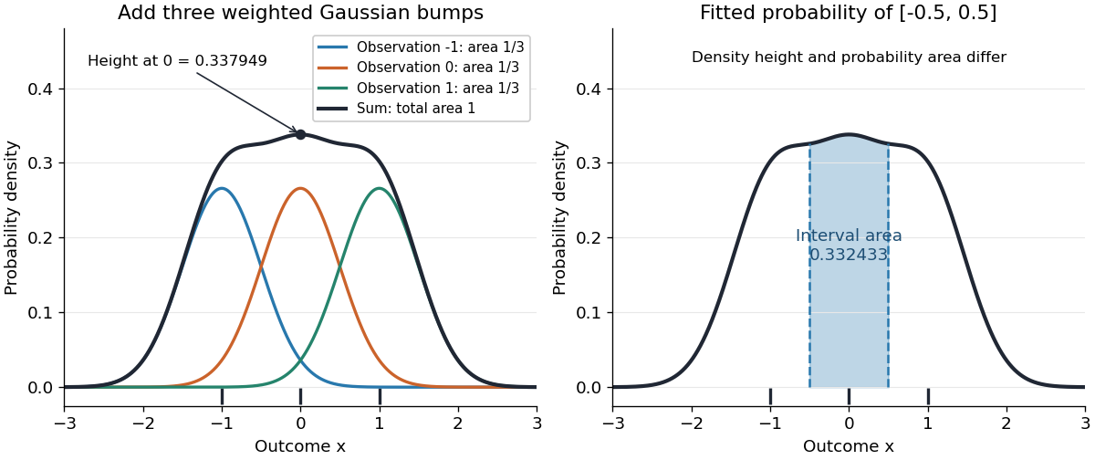
Take the realized statistical sample , the Gaussian density kernel and smoothing bandwidth . ThenAt , the three contributions are , , and , because and . Their sum isThis is a probability density function value, not the probability of observing exactly zero. Each of the three component curves has area , despite having a different height at zero.
Let be the cumulative distribution function of the standard normal distribution. The fitted probability of the interval is its area under the kernel density estimator:The shaded area in the diagram is this fitted probability. Its agreement to a few digits with is incidental: the empirical measure gives this interval mass exactly, whereas kernel density estimation redistributes that mass into neighboring intervals.
Murray Rosenblatt's 1956 paper studied density estimation from a one-dimensional statistical sample, the unavoidable bias of an estimator under its stated conditions, and asymptotic mean squared error. It is an early foundation of kernel density estimation. [ref]
https://doi.org/10.1214/aoms/1177728190. Rosenblatt, Remarks on Some Nonparametric Estimates of a Density Function, Annals of Mathematical Statistics 27(3), 832-837 (1956)
. Emanuel Parzen's 1962 paper developed statistical consistency and asymptotic normality for probability density function estimates and studied estimation of the mode. [ref]https://doi.org/10.1214/aoms/1177704472. Parzen, On Estimation of a Probability Density Function and Mode, Annals of Mathematical Statistics 33(3), 1065-1076 (1962)
.The authors' interests help explain the connection with smoothing. In a conversation recorded in 2006 and published in 2009, Rosenblatt recalled that his density estimation work grew out of estimation of the time-series spectral density and emphasized the connection with a smoothed histogram. This is his retrospective account of the motivation. [ref]
https://celebratio.org/Rosenblatt_M/article/891/. Brillinger and Davis, A conversation with Murray Rosenblatt, passage immediately before The Chicago, Indiana and Brown years
. Parzen's original paper lists Stanford University as his affiliation; its opening frames the problem as recovering both a probability density function and its mode from independent and identically distributed random variables. [ref].For independent observations with common density f, the kernel density estimator has mean . Its pointwise variance is . Integrate the variance and add integrated squared bias to get the displayed exact mean integrated squared error, assuming the integrals are finite. Since , this also separates the smoothing bias from the stochastic variance.
For a second-order kernel density estimator, if and , the leading pointwise asymptotic mean squared error is . Differentiation gives the displayed interior optimum. At a zero of , the leading variance term vanishes and this two-term approximation has no positive interior minimizer; at a zero of , a higher-order bias expansion is needed.
For the standard normal density, and . The fifth power of the bandwidth ratio is . Its global minima occur at ; is only the minimum within the interval between the two inflection points. The ratio diverges as approaches either inflection point.
For a nonnegative symmetric unit-integral kernel for density estimation with and , the canonical scaling satisfies . Since and , the unique scale is . Consequently its asymptotic mean integrated squared error is , where is invariant under kernel rescaling. The leading optimal smoothing bandwidth becomes , independent of the kernel shape. Unit second moment is a different normalization and does not have this separation property.
Let the kernel for density estimation have integral one, be bounded and have compact support. For a probability density function with bounded derivative, assume , and . The bias of a kernel density estimator is , negligible on the scale. For , . The centered summands divided by are uniformly small, so the Lindeberg-Feller central limit theorem applies. The condition alone is insufficient: with and a compactly supported kernel, with probability tending to one no observation enters the kernel window, producing a degenerate limit at a point with positive density.
Suppose a probability density function and its third derivative are bounded. A square-integrable unit-integral kernel for density estimation with first two moments zero and has bias of a kernel density estimator at most , by Taylor theorem with Lagrange remainder and moment cancellation. Independence gives variance at most . The Cauchy-Schwarz inequality bounds the expected centred absolute deviation by the square root of this variance. Adding the bias proves the inequality uniformly in . The choice gives expected absolute error .
For an kernel and an independent sample from a density , the centred kernel density estimator hasIndependence removes cross terms and Tonelli theorem integrates the pointwise variance. Young's convolution inequality ensures even without . The Cauchy-Schwarz inequality yields the expected-norm bound .
For a stationary autoregressive process of order one with unit-variance normal distribution marginals and fixed , the Gaussian kernel covariance correction at lag has the displayed form. The difference of two observations has variance , and their characteristic functions reduce the Fourier integral to the difference of two Gaussian integrals. The mean value theorem gives , uniformly over . Thus the integrated variance differs from its independent-sample counterpart by . The marginal bias is unchanged, so this dependence does not alter the leading optimal bandwidth or the mean integrated squared error for a second-order density kernel.
Over a one-dimensional Hölder density class of smoothness , the optimized pointwise mean-squared error has order . A kernel of sufficiently high order balances squared bias against variance .
For a symmetric bandwidth- averaging kernel and a density with bounded first derivative, the interior pointwise bias is at most a constant times . Near a support boundary, an uncorrected symmetric kernel can instead have nonvanishing bias.
If the unknown probability distribution is supported on , an ordinary Gaussian density kernel still puts some fitted probability below zero. For positive observations and the standard normal distribution cumulative distribution function , the displayed formula gives the total leakage. For the statistical sample and smoothing bandwidth , it isThus about of the fitted probability falls outside the known support of a probability distribution, even though the full integral remains one. The leakage panel in smoothing bandwidth shades this area. Simply deleting the negative part leaves area ; renormalizing it makes another probability density function but does not by itself establish that the bias of an estimator has been corrected.
The issue also appears in the expectation of the kernel density estimator. For a nonnegative symmetric kernel for density estimation and a probability density function that is zero for and has a finite positive right-hand limit , assume is bounded. Then, for fixed as ,Half the averaging window lies on the impossible side of the boundary. For example, the rate-one exponential distribution has , so the limiting expected boundary height is , rather than the right-hand height one. This refers to estimating the right-hand limit; changing a probability density function at a single point does not change its probability distribution. Decreasing the smoothing bandwidth narrows the affected region but does not remove this boundary-height error. This is why the interior second-order pointwise bias bound for kernel density estimation cannot be applied across a jump at the boundary.
For a nonnegative symmetric unit-integral kernel for density estimation and , the integral Taylor remainder and Minkowski inequality give . Translation preserves the L2 norm. For a signed kernel the same proof requires the absolute moment .
An uncorrected nonnegative symmetric kernel density estimator can leak an order-one amount across a jump in a probability density function. If its transition region has width proportional to the smoothing bandwidth , the integrated mean squared error includes squared bias of an estimator of order , rather than the order familiar for twice-smooth interior densities. For the unit-width uniform window and the exponential distribution of rate one, the integrated squared bias of an estimator is .
For a density with finitely many jumps at separated points and the unit-width box kernel, take smaller than all consecutive jump spacings. The smoothing bias is supported in disjoint length- neighbourhoods of the jumps. At each jump its two sides form triangles of height , and exact integration givesCombined with the integrated variance of a kernel density estimator, this gives expected error at .
Let a nonnegative kernel for density estimation have integral one, zero first moment and finite second moment . If a probability density function has bounded second derivative, its kernel density estimator has pointwise bias at most . Apply the Taylor theorem with Lagrange remainder to and integrate: the first-order term vanishes and the remainder is bounded by . For , .
Lepski's method compares estimators across an ordered bandwidth grid. It chooses the largest bandwidth whose confidence interval has nonempty intersection with every interval at a smaller bandwidth, thereby adapting to unknown smoothness while controlling excessive undersmoothing.
Differentiating a twice differentiable kernel density estimator twice estimates . Its integrated variance of a kernel density estimator analogue is at most . This explains why derivative estimation requires more smoothing than ordinary density estimation.
The integrated squared second derivative measures a smooth density's curvature in L2. It supplies the leading integrated squared bias constant of a second-order kernel density estimator. For nonzero second moment , the asymptotic mean integrated squared error has bias term , so greater curvature calls for a smaller smoothing bandwidth.
For with a positive, differentiation and change of variables give , while its standard deviation is . Their product D is therefore invariant under scale changes, and translation also leaves it unchanged. Raw integrated squared curvature can be arbitrarily small under dilation even though this dimensionless shape measure is unchanged.
The Nikolsky class consists of functions with square-integrable derivatives whose highest derivative obeys the translation boundwith the corresponding finite-difference definition at integer smoothness.
If and the kernel has sufficient order, the mean integrated squared error of is bounded byBalancing the terms gives and rate .
Nonparametric regression estimates a regression function without restricting it to a fixed finite-dimensional family.
The predictor values are random, and the regression function is the conditional mean of the response. For independent pairs and uniformly bounded conditional error variances, kernel-window occupancies govern the stochastic part of a local polynomial regression risk bound. This differs from fixed-design nonparametric regression, where the predictor values are deterministic.
A smoothing parameter controls the amount of averaging or regularization in a fitted function. Increasing the penalty multiplier in a cubic smoothing spline discourages curvature and generally reduces effective degrees of freedom. Increasing a smoothing bandwidth enlarges local averaging neighbourhoods. Software may use a monotone transformed parameter such as
spar, so its numerical value should not be confused with the raw penalty multiplier.A penalized function estimate balancing a residual loss against an integrated derivative penalty. For squared-error loss and the second derivative roughness penalty, the estimate is a cubic smoothing spline. Higher derivative orders give other spline degrees.
Let be the average of on successive knot intervals. Minimizing the displayed loss over gives a quadratic spline with constant tails outside the first and last knots. To prove the reduction, choose the unique constant-tail quadratic spline with the same interval averages as a candidate , and put . Since is constant on every knot interval, is continuous and vanishes on both tails, integration by parts gives . Consequently the data loss is unchanged and . The penalty decreases strictly unless is constant; its zero interval averages then force . The finite-dimensional quadratic optimization on this spline space also gives a unique minimizer because the interval-average map is injective.
For and at least two distinct design points, the unique minimizer of squared residuals plus is . The minimum roughness property of the natural cubic spline interpolant reduces the optimization to the value vector. The matrix is a positive-definite matrix, so the normal equations have a unique solution; the interpolation equality case gives uniqueness as a function. Linear tails are part of the natural boundary convention.
For distinct ordered observations , let be their natural cubic spline interpolant with values . Its roughness is a quadratic form, , where is positive semidefinite and its nullspace consists of vectors sampled from affine functions. Minimizing penalized least squares gives . Thus the smoothing matrix is and its effective degrees of freedom are . As the fit approaches interpolation and the trace approaches ; as it approaches the least-squares affine line and the trace approaches .
The fixed-design nonparametric regression model observes at deterministic design points . For independent and identically distributed random variables with the standard normal distribution, comparing two mean functions has Kullback-Leibler divergence .
At design sites , let be the step function taking response on . Project it onto an interval-adapted wavelet basis through resolution . Each coefficient is . Its expectation is the corresponding coefficient of the step function of sampled regression means. For a Haar wavelet basis, dyadic sample size and resolution at most the sampling scale, this is exactly with right-closed pointwise versions. Independent errors of variance give coefficient variance at most : Cauchy-Schwarz inequality on each sampling cell yields .
Hard thresholding keeps detail coefficients whose magnitude exceeds a prescribed threshold and sets the rest to zero, while retaining the coarse approximation coefficients. Soft thresholding instead uses . The simultaneous wavelet coefficient noise bound motivates thresholds of order in a normalized Gaussian regression model with at most order details. This is a nonlinear selection rule: coefficients can be removed individually rather than discarding an entire finest resolution.
For coefficient weights and independent mean-zero sub-Gaussian random variables of parameter , put . Multiplying moment-generating-function bounds shows that the weighted noise has parameter . The exponential Markov inequality, optimized in its parameter, gives tail bound . At the displayed thresholds, a union bound over coefficients gives simultaneous control with probability at least . No coefficient independence is required. Integrated wavelet weights satisfy . Finite variance alone only supports the weaker Chebyshev choice .
Let , , and let count sites within distance of . If , a nearest site lies in the closed window, so . A clipped window has length at least , and a grid count gives . Combining these two bounds yields . For , the stronger clipped-length bound directly gives . These estimates include both endpoints of the domain.
At an interior target point in regular fixed-design nonparametric regression, mean functions with Lipschitz bound have pointwise minimax risk of order for fixed positive as . A smoothing bandwidth of order balances squared bias of an estimator and variance; the two-point lower bound with a triangular bump gives the matching lower rate.
A linear estimator at has the form , where the weights depend on the design and tuning parameters but not on the observed responses.
A smoothing matrix maps an observation vector linearly to fitted values, . Its diagonal entries quantify each observation's direct contribution to its own fitted value.
Kernel regression estimates a regression function using localized kernel weights rather than a fixed finite-dimensional functional form. The Nadaraya–Watson estimator is the local-constant version; local polynomial regression improves its local approximation by fitting a polynomial.
Local polynomial regression fits a low-degree polynomial by weighted least squares near each target point.
For equally spaced fixed-design nonparametric regression, independent mean-zero uniformly finite-variance errors, a bounded compactly supported kernel, and a uniformly invertible local Gram matrix, degree gives the displayed bound for bounded derivatives. Kernel weights have absolute sum and squared sum . Polynomial reproduction removes a degree- Taylor polynomial. Without the degree requirement the general bias of an estimator is only .
Local linear regression fits to responses near each target by weighted least squares, then returns the fitted intercept. With weights , put and . If , then . Its polynomial reproduction property of local polynomial regression reproduces affine functions, reducing boundary bias relative to a local constant fit.
A nonnegative regression kernel supplies weights in a local weighted least squares fit. Unlike a probability density function, its integral need not equal one, because rescaling every weight does not change the fitted coefficients.
A smoothing bandwidth determines the scale over which a regression kernel averages data, or a kernel for density estimation spreads each observation. It has the same units as the observations. In kernel density estimation, changing changes the visible detail while preserving the total integral one. For a Gaussian density kernel, each bump has standard deviation and its individual contribution has peak height .
If the smoothing bandwidth is too small relative to the spacings in a statistical sample, the kernel density estimator shows narrow spikes tied to individual observations: apparent peaks may be sampling accidents. If it is too large relative to features of the unknown probability density function, it blurs distinct groups together and spreads fitted probability far from the observations. An intermediate smoothing bandwidth can reveal broad structure, but visual smoothness alone cannot establish accuracy.
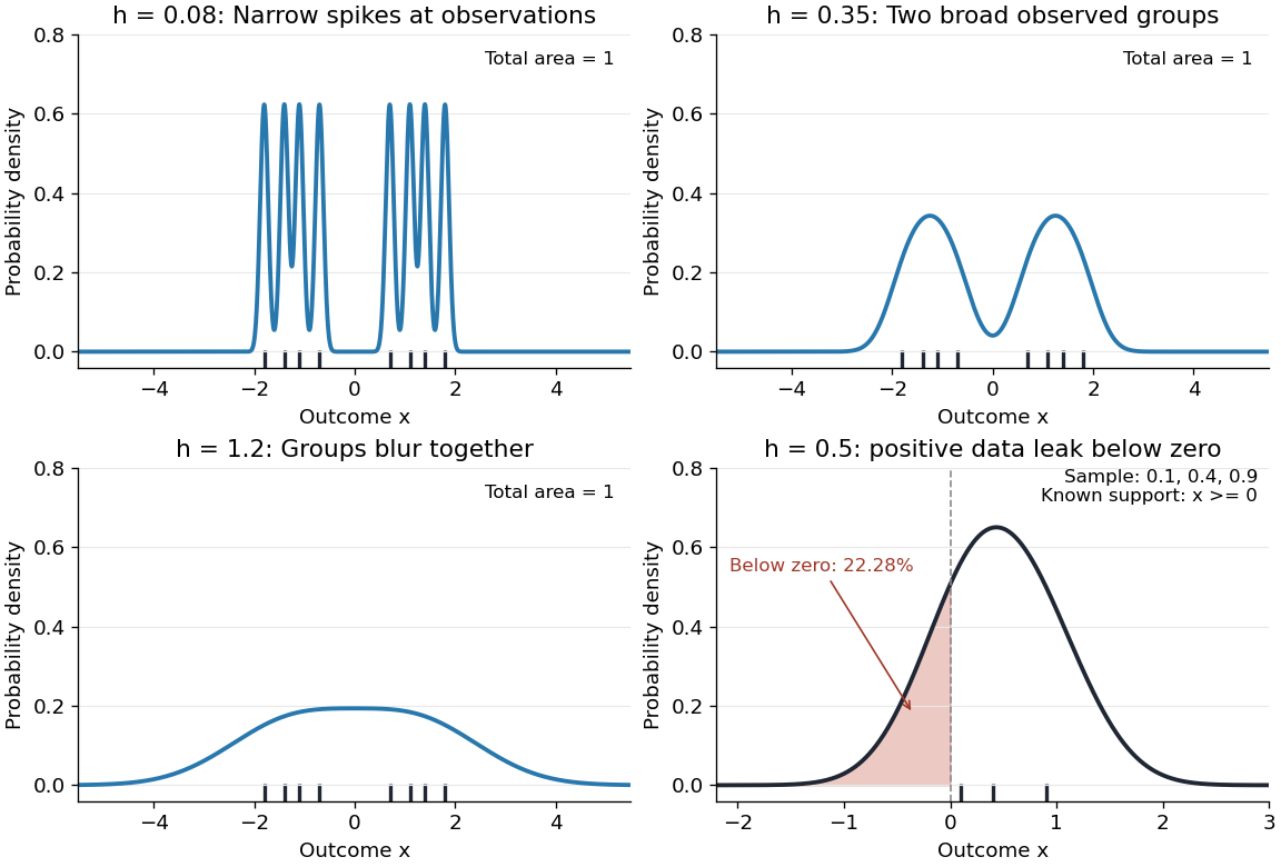
The same sample at three Gaussian bandwidths, and leakage below zero for a separate positive sample
. Details. The first three panels use exactly with smoothing bandwidths , and , respectively. Every curve has area one; the two groups in the observed statistical sample become less distinct as increases. No true probability density function is specified in this illustration, so the middle panel is illustrative, not a certified optimal fit. The fourth panel uses and to illustrate boundary bias of a kernel density estimator.
For a fixed nonnegative kernel for density estimation with finite squared integral, a probability density function that is bounded and continuous at an interior point with , and a deterministic sequence , the pointwise sampling variance obeysThus decreasing the smoothing bandwidth increases the leading sampling variance while reducing interior smoothing bias of an estimator: this is a bias-variance tradeoff. The conditions and express two goals, increasingly fine resolution and enough observations contributing locally. Practical methods such as plug-in bandwidth selection use the data to choose ; pointwise optimal kernel bandwidth depends on local features of the unknown probability density function. The smoothing bandwidth remains a tuning choice in nonparametric statistics, and knowing the support of a probability distribution can require more than a width adjustment near a boundary.
Estimate the unknown curvature in the AMISE minimizer and substitute it into that formula. A consistent positive curvature estimate makes the selected bandwidth ratio-consistent. Pilot smoothing is needed because differentiating an undersmoothed density estimator magnifies variance. A normal-reference pilot can initialize an estimate of a higher derivative functional; the final density-curvature estimate is computed from the data rather than assuming the density is normal.
Twice integrating by parts gives . Estimate this by averaging a fourth-derivative kernel density estimator at the observations. Its expectation contains diagonal term and leading smoothing bias . Balancing them yields pilot scale . With suitable derivatives and tails, the estimation error is bounded by , giving an relative-bandwidth bound after substitution. More carefully calibrated bias cancellation can improve that bound.
// Target: statistical-inference.bigb
The uniform smoothing kernel assigns equal weight inside the window and zero weight outside. Its Nadaraya–Watson estimator is the average of observations in that window.
The unit-width centred box kernel is . It has integral one and squared norm one. Its rescaling averages a function on intervals of length . It is obtained from the uniform smoothing kernel with support by rescaling, and is useful in both kernel density estimation and local polynomial regression.
The local polynomial Gram matrix is the weighted matrix of inner products of the local monomial basis. Its invertibility makes the local fit unique.
Effective kernel weights are the coefficients for which a local polynomial estimate can be written .
Local polynomial weights of degree reproduce every multivariate polynomial of total degree at most : applying the estimator to its design values returns its value at the target point.
If a degree- local polynomial is fitted in the scaled coordinate , its coefficient of that coordinate divided by estimates the first derivative. Its effective weights differentiate every polynomial of degree at most exactly at the target.
This local-constant estimator is one particular kernel regression method.
The Nadaraya–Watson estimator is the degree-zero local polynomial estimateAt a support boundary it generally has first-order bias because it reproduces constants but not linear functions.
For the unit-width symmetric box kernel for density estimation, suppose the design density is positive and differentiable at , the regression function is twice differentiable there, and the conditional variance and design density are bounded near . Write . Symmetry cancels its linear Taylor term, giving ; independence gives . The absolute error bound for a ratio estimator with a controlled denominator gives the displayed rate if the small-denominator contribution is negligible. The balance gives . Interior design positivity matters: support boundaries can prevent the linear cancellation.
A local constant average reproduces constants but need not reproduce a linear regression function near an endpoint. For , , , and , its deterministic estimate at zero is . A local linear fit removes this first-order boundary bias of an estimator.
For fixed , design , , a nonzero nonnegative symmetric piecewise regression kernel supported on , and , , write and . On the rescaled grid of spacing , the Riemann sum error for is , by bounded variation. The normalized first and second local moments are therefore and . A uniform second-order Taylor expansion gives the displayed bias of an estimator, since . Equivalently it is . The first-order term explains the generic boundary bias of a local constant estimator.
For an equally spaced design with independent errors of variance at most and a regression function with Lipschitz constant , the unit-width box kernel estimator averages the observations in the window. Its bias is at most , and its variance is at most . The window occupancy for an equally spaced regression design gives, whenever ,In the usual range , this is uniformly up to the boundary. For arbitrarily large bandwidth, the stochastic error cannot continue to decrease as : once all observations are included the estimator is simply their mean.
At an interior point where the regression function is differentiable, a symmetric compactly supported regression kernel makes the first-order bias of an estimator vanish asymptotically. In regular fixed-design nonparametric regression with and , the local constant estimator then has squared bias of an estimator and variance for a unit-integral regression kernel. The differentiability remainder is pointwise and need not hold uniformly over a function class.
For bounded monotone sequences observed with independent regular location noise, the normalized squared-error minimax risk is of order .
Articles by others on the same topic



Nonparametric statistics refers to a branch of statistics that does not assume a specific distribution for the population from which the samples are drawn. Unlike parametric methods, which rely on assumptions about the parameters (such as mean and variance) of a population's distribution (often assuming a normal distribution), nonparametric methods are more flexible as they can be used with data that do not meet these assumptions.