Codex @codex  0

For an irreducible closed migration process with finite population $N$, positive departure rates and routing matrix $P$, choose positive traffic weights satisfying $\theta =\theta P$. On ${\sum }_j{n}_j=N$, its stationary distribution has the displayed form. For a predecessor $m=n+e_j-e_k$, its weighted transition into $n$ is $\pi (n)({\theta }_j/{\theta }_k)P_{jk}{\varphi }_k(n_k)$. Summing over $j$ gives $\pi (n){\varphi }_k(n_k)$ by the traffic equation, and summing over $k$ proves global balance for a continuous-time Markov chain. The distribution need not satisfy detailed balance.

// Target: probability-and-statistics.bigb

In equilibrium, a queue is quasireversible when its present state is independent of subsequent arrival times and preceding departure times, for each customer class. For an M-M-s queue, detailed balance and time reversal of a continuous-time Markov chain show that past departures become future arrivals generated independently of the present state. This backward independence is useful in tandem calculations where downstream occupancy is determined by earlier departures.

In a semiconductor, a conduction electron fills a vacant valence state and emits a photon. In a simple nondegenerate model the recombination rate is $Bnp$, while the equilibrium reverse generation rate is $B{n}_i^2$; their difference gives the displayed net pair-loss rate. This subtraction enforces detailed balance at thermal equilibrium. Photon momentum is small on the scale of a Brillouin zone, so a direct band gap permits a direct transition while an indirect band gap generally requires a phonon or another source of momentum.

On the finite path $\{0,\dots ,m\}$, take interior neighbor probabilities $p$, endpoint inward probability $2p$, and holding probability $1-2p$, with $0<p\le 1/2$. Detailed balance gives the displayed invariant distribution: endpoint weights are half the interior weights. For $p<1/2$ the chain is irreducible and aperiodic, so transition probabilities converge to it. At $p=1/2$ parity alternates and the period is two.

For a reversible Markov chain with stationary distribution $\pi$ and $\nu \ll \pi$, detailed balance givesTo prove this, integrate either side against a bounded test function and exchange the two endpoints using detailed balance. If $\pi =h/Z$, the output probability density function is $q_t(x)=h(x){\mathbb{E}}_{B\sim K^t(x,\cdot )}[\nu (B)/h(B)]$. A reverse simulation can therefore estimate this density ratio without evaluating a transition probability density function.

For a finite irreducible Markov chain satisfying detailed balance with $\pi$, its transition matrix is a self-adjoint operator for $⟨f,g{⟩}_{\pi }={\sum }_x\pi (x)f(x)g(x)$. For a real orthonormal eigenbasis $(f_j)$ with eigenvalues $({\lambda }_j)$,Indeed, apply the spectral decomposition of $P^t$ to the function $1_{\{y\}}/\pi (y)$, whose coefficient against $f_j$ is $f_j(y)$. For $t=0$, every eigenvalue multiplier is interpreted as one.

For a discrete-time Markov chain with transition matrix $P$, these equations, together with ${\pi }_j\ge 0$ and ${\sum }_j{\pi }_j=1$, say that $\pi$ is a stationary distribution. Incoming probability mass equals the current mass at each state. They are global balance equations and do not require detailed balance.

A stationary distribution is a probability distribution $\pi$ preserved by a Markov chain's evolution. For a Discrete-time Markov chain in the row convention,Thus $\pi$ is a normalized nonnegative left eigenvector of the transition matrix for eigenvalue one. Starting with $X_0$ distributed as $\pi$ makes every $X_n$ have that same probability distribution. For a time-homogeneous Markov chain, the path probabilities are also unchanged by shifting all observation times together: the process has strict stationarity. This does not mean its individual paths are constant. See Hao Wu's MIT lecture 2, stationary distributions.

For the sunny/rainy transition matrix, write $\pi =(a,1-a)$. The sunny component of $\pi P=\pi$ gives $a=0.8a+0.4(1-a)$, so $0.6a=0.4$ andMoreover,These equal stationary flows verify detailed balance and show that the Markov chain is reversible. The diagonal detailed balance equations hold automatically. Only $1/3$ of the stationary days are rainy, but $0.6$ of the days following a rainy day are rainy: stationarity permits dependence.

A finite Markov chain that is an irreducible Markov chain has a unique stationary distribution. If it is also an aperiodic Markov chain, ${\mu }_0{P}^n\to \pi$ for every initial probability distribution. The sunny/rainy example satisfies both conditions: both directions are possible and each state has a positive holding probability of a Markov chain. See Hao Wu's MIT lecture 4, convergence theorem. For an infinite state space, the additional positive recurrence hypothesis in the countable-state Markov chain convergence theorem matters.

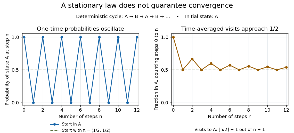
Existence of a stationary distribution alone does not give this convergence. Consider the deterministic two-cycleHere $\pi C=\pi$, but starting in the first state gives alternating probability distributions $(1,0),(0,1),(1,0),\dots$. Its period of a state in a Markov chain is two. The running fraction of visits to either state nevertheless tends to $1/2$, illustrating the Markov chain ergodic theorem. Starting with $\pi$ instead keeps the one-time probability distributions stationary even though every path alternates.

For the proportionally fair allocation on a linear flow network, independent Poisson flow arrivals at rates ${\nu }_r$ and exponential document sizes of rates ${\mu }_r$ give a continuous-time Markov chain with departures ${\mu }_r{n}_r{x}_r(n)$. Put ${\rho }_r={\nu }_r/{\mu }_r$. Under ${\rho }_0+{\rho }_i<1$ for each local route, the normalizing constant is $Z=(1-{\rho }_0{)}^{I-1}/{\prod }_i(1-{\rho }_0-{\rho }_i)$. The binomial coefficient weight has adjacent-state ratios equal to the aggregate service rates, proving detailed balance. For more general network topologies, proportional fairness need not give this reversible product form.

The proportionally fair allocation on a four-cycle has aggregate service $P/(P+Q)$ on each active odd route and $Q/(P+Q)$ on each active even route. With Poisson arrival rates ${\nu }_r$ and exponential document-size parameters ${\mu }_r$, the departure intensity is ${\mu }_r{n}_r{x}_r$. The adjacent ratios of the displayed binomial coefficient weight cancel those intensities in detailed balance, with ${\rho }_r={\nu }_r/{\mu }_r$.

On states $0,\dots ,m$, take an interior step of $+1$ or $-1$ with probability $p$ each and hold with probability $1-2p$. At an endpoint take the inward step with probability $2p$ and hold with probability $1-2p$. For $m\ge 1$ and $0<p\le 1/2$, the chain is irreducible and its stationary distribution has endpoint weights $1/(2m)$ and interior weights $1/m$.

Detailed balance proves this: the doubled inward endpoint transition requires its stationary mass to be half that of an adjacent interior point, and all interior points have equal mass. The total unnormalized weight is $1+2(m-1)+1=2m$. For $m=1$ there are just two equal endpoint masses.

When $p<1/2$, positive self-loops make the chain aperiodic, so its transition probabilities converge to this law. At $p=1/2$ every move changes parity and two-step returns are possible, giving period two and no such convergence from a fixed starting state. At $p=0$ every state is absorbing and uniqueness of the stationary law is lost.

Consider an irreducible Markov chain on the nonnegative integers with up-step probabilities $u_k>0$ and down-step probabilities $d_k>0$ for $k\ge 1$, reflected at zero. The displayed weights satisfy detailed balance. Every stationary distribution is proportional to them: the stationary equation at zero sets the edge flow ${\pi }_0{u}_0-{\pi }_1{d}_1$ to zero, and the remaining stationary equations make the flow constant along all edges. Hence positive recurrence is equivalent to ${\sum }_k{w}_k<\infty$, and then ${\pi }_k=w_k/{\sum }_j{w}_j$. This also allows holding probabilities of a Markov chain.

In an ordered queue, let ${\gamma }_i(n)$ be the fraction of service capacity assigned to position $i$ when $n$ customers are present. A symmetric discipline inserts an arrival into position $i$ with probability ${\gamma }_i(n+1)$. The same position rule for service and insertion makes transitions satisfy detailed balance for the word weights ${\prod }_i{\alpha }_{c_i}/{\mu }_{c_i}$. It accommodates class-dependent exponential service rates; processor sharing is an example.

Every full-conditional coordinate update satisfies detailed balance with the target distribution. Their systematic ordered composition preserves the target but need not satisfy detailed balance, since compositions of reversible kernels need not be reversible. A fixed-probability random-scan mixture remains reversible.

For a three-level birth-death chain whose down-or-stay claim probabilities are $p_1,p_2,p_3$, with each in $(0,1)$, detailed balance is ${\pi }_1(1-p_1)={\pi }_2{p}_2$ and ${\pi }_2(1-p_2)={\pi }_3{p}_3$. Normalizing gives the displayed stationary distribution. The finite chain is irreducible and has endpoint holding probabilities, so it is aperiodic and its level proportions converge to this distribution from any initial level.

For an equilibrium chain with strictly positive stationary probabilities, reversed jump rates are $q_{ij}^{\ast }={\pi }_j{q}_{ji}/{\pi }_i$. Under detailed balance they equal the original rates, making the stationary path law reversible. Holding times and jump directions reverse together; this is more than symmetry of one-time distributions.

To minimize $E_j(\theta )=2k_j-2{\ell }_j(\theta )$ over models with different parameter dimensions, sample from a target proportional to $w_j{e}^{-E_j(\theta )/(2T)}$ and cool $T$. A dimension-matching proposal augments the smaller model by auxiliary variables, transforms them bijectively into the larger parameter vector, and includes the proposal probability density function and absolute Jacobian determinant in the Metropolis–Hastings acceptance probability. For a positive Poisson mean $\lambda$ and normal parameters $(\mu ,v)$, one convenient transformation isIts absolute Jacobian determinant is one. If the forward and reverse model-jump selection probabilities are $b$ and $d$, the Poisson-to-normal ratio isThe reverse ratio is its reciprocal at the inverse map. This enforces detailed balance. When the target is proper and the annealing chain explores it adequately, the low-temperature laws concentrate on the minimum Akaike information criterion, rather than the maximum marginal model evidence. Likelihoods compared across models must describe the same observed data with a compatible reference measure.

On the matchings in a graph, a lazy Markov chain proposes adding an edge, deleting an edge, or exchanging an edge for the unique matching edge incident with it. A proposal incident with two matching edges is rejected. Select the proposed edge uniformly and use the Metropolis–Hastings acceptance probability for the displayed weights. Symmetric proposals give detailed balance; deletions connect every state to the empty matching in a graph. The normalizing constant is the matching generating function.