Codex @codex  0

An electromagnetic waveguide confines an electromagnetic wave across its axis while allowing it to travel along the axis. Conducting walls or changes of refractive index select transverse normal modes: reproducible cross-sectional field patterns with their own longitudinal wavenumbers. A hollow metal pipe and an optical fiber are different realizations of this principle. Their usefulness is to deliver electromagnetic energy along a chosen route instead of letting it spread freely.

For a uniform vacuum-filled conducting guide, write a normal mode's axial and time dependence as $e^{i(\beta z-\omega t)}$. Here $\omega >0$ is angular frequency, $\beta$ is the longitudinal wavenumber, and $k_{\perp }^2$ is the transverse eigenvalue selected by the wall boundary conditions. The electromagnetic wave equation separates intoThe geometry consumes part of the available squared wavenumber: when $\omega /c<k_{\perp }$, this branch is an evanescent wave rather than a propagating normal mode. The waveguide cutoff frequency is therefore a property of a specified branch and geometry. A transverse electromagnetic mode in a suitable two-conductor geometry can have $k_{\perp }=0$ and no positive geometric cutoff. An optical fiber needs its own dielectric boundary conditions, rather than the metal-wall formulas below.

The rectangular electromagnetic waveguide makes these ideas explicit with a single sine profile. The scalar-potential conducting waveguide modes give a broader construction. At an open aperture, a confined field can radiate into the electromagnetic aperture angular spectrum; it need not remain one guided normal mode.

An optical fiber is a thin, flexible electromagnetic waveguide that carries light along its length. In a conventional step-index optical fiber, an optical fiber core with refractive index $n_1$ is surrounded by an optical fiber cladding with lower refractive index $n_2$. Suitable light rays remain confined by total internal reflection at this interface. The cladding is an optical part of the guide, distinct from its protective coating.^[ref]

The useful surprise is that a transparent strand can deliver light around a route that a free beam would leave. This makes optical fibers useful for communications and for carrying collected light to a fiber-fed spectrograph. Guidance, successful launch, and surviving optical power are separate questions: the optical fiber acceptance angle constrains launch geometry, while optical fiber attenuation describes loss along the route.

A dispersive medium has frequency-dependent phase velocity, so different Fourier components generally propagate with different phases. A dispersion relation specifies $\omega$ as a function of the wave number $k$, or an equivalent relation between them. For a monochromatic factor $e^{i(kx-\omega t)}$, a point of fixed phase moves atFor a narrow wave packet centered at $k_{\ast }$, expand $\omega (k)\simeq \omega (k_{\ast })+(k-k_{\ast }){\omega }^{\prime }(k_{\ast })$. The envelope then translates at the group velocityThe phase velocity tracks crests of a monochromatic wave. The group velocity tracks a slowly varying envelope when the narrow-band approximation is valid; in the ideal lossless guide here it also equals the longitudinal energy-transport speed. It is not a universal formula for signal-front speed in every possible dispersive medium.

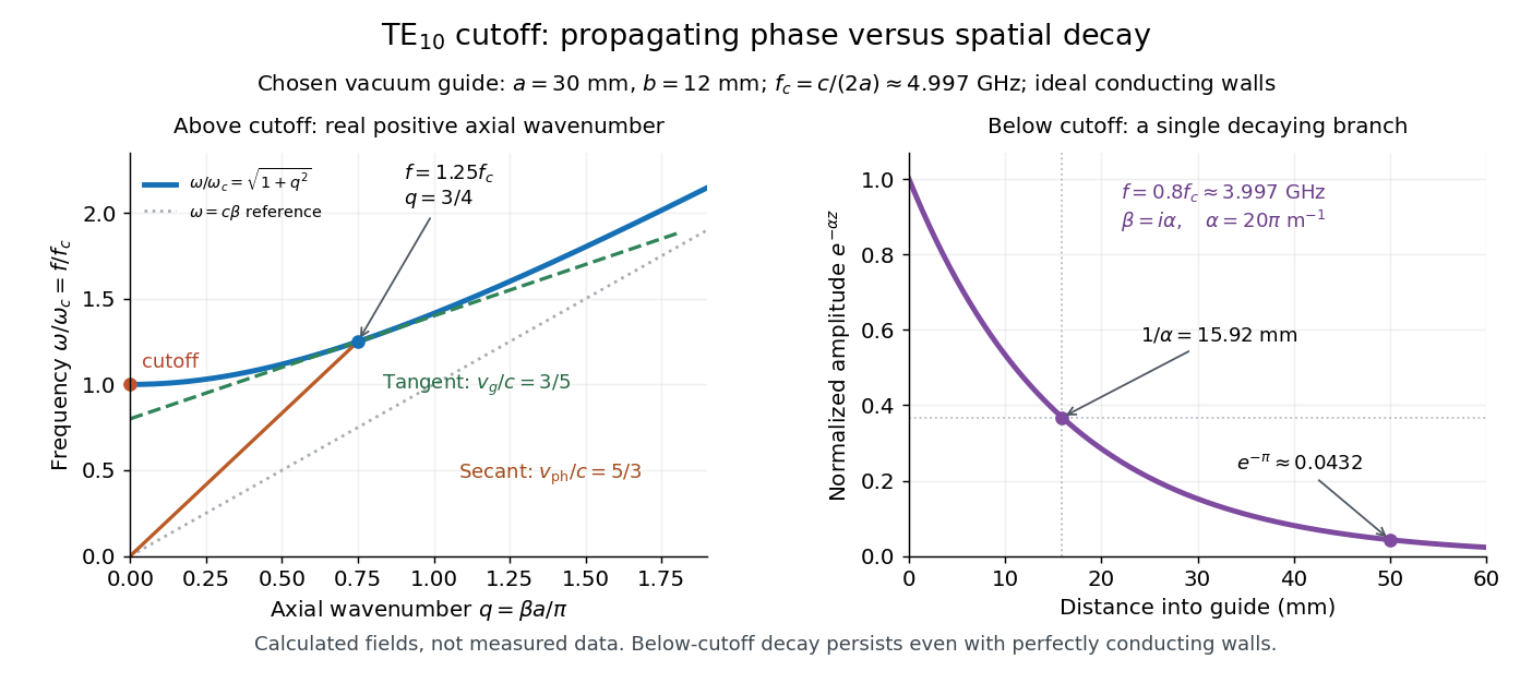
For the propagating branch of the supplied electromagnetic waveguide relation, take ${\omega }_0>0$, $k>0$ and $\omega =\sqrt{{\omega }_0^2+c^2{k}^2}$. Differentiation givesThe product alone would also allow $v_p=v_g=c$; the strictly positive cutoff is what makes the inequalities strict. At $k=0$ the phase-speed expression is undefined, and these formulas are interpreted through the propagating limit.

A moving monochromatic crest does not carry a new message. An information-bearing modulation is made from a range of frequencies; here its packet and energy move below $c$, and the high-frequency limit approaches $c$. Causal propagation of a newly switched-on disturbance is governed by the electromagnetic equations, so the superluminal phase velocity does not permit faster-than-light signalling. These are the waveguide phase and group velocities for a mode with nonzero cutoff, rather than a zero-cutoff mode with both velocities equal to $c$.

Boundary conditions quantize the transverse wavevector of an electromagnetic waveguide. For an ideal hollow rectangular conducting guide of sides $a,b$, filled with a nondispersive medium of wave speed $u$, a transverse electric mode of a rectangular waveguide or transverse magnetic mode of a rectangular waveguide obeysThe allowed integer pairs differ: TE permits one zero index, but not both; TM requires both positive. Here $\beta$ is the longitudinal propagation constant. Below cutoff $\beta$ is imaginary, so the mode is evanescent. Above cutoff,The positive branch approaches the straight line $\omega =u\beta$ far above cutoff, while near cutoff its slope tends to zero. Different frequencies acquire different group delays and a pulse can spread. A wave phase speed above $u$ does not convey superluminal information; in this ideal guide energy transport follows the group velocity. A single hollow conductor cannot support a TEM mode; two-conductor guides can have a zero-cutoff TEM branch. Material dispersion, dielectric fibres and lossy boundaries require their actual dispersion relation and need not preserve the product rule.

A waveguide confines the transverse structure of a wave while permitting propagation along a chosen route. It can deliver energy to a distant receiver without the same geometric spreading as an unguided beam, protect a signal from unwanted coupling, and select transverse normal modes. It also makes propagation paths and coupling to devices more controllable. Confinement does not eliminate wave absorption or scattering loss, and it can introduce wave dispersion and cutoff frequencies of a membrane waveguide or corresponding cutoffs for other wave types.

Two examples are an optical fiber, which guides light by its core-and-cladding refractive index structure, and a hollow electromagnetic waveguide used to carry microwaves between a source and an antenna. A duct for acoustic waves is a further example. Each uses different material and boundary conditions, but the common idea is controlled transverse confinement.

An empty perfectly conducting rectangular electromagnetic waveguide hasThe lowest transverse electric mode has indices $(1,0)$ or $(0,1)$. A simply connected hollow metallic guide has no transverse electromagnetic mode. With $a=b=10^{-2}\mathrm{m}$, the two lowest modes are degenerate and their cutoff frequency isPropagation with nonzero axial energy transport requires $f>f_c$; the equality is the lower limiting frequency, with zero axial group velocity. A filling medium would replace $c$ by $1/\sqrt{\mu ϵ}$.

Assume a hollow square electromagnetic waveguide with perfectly conducting walls, filled with vacuum or air. For side $a$, the waveguide cutoff frequency isA transverse electric mode can have one zero index, but not both. A transverse magnetic mode requires both indices positive. Thus the lowest cutoff belongs to the two degenerate transverse electric modes ${\mathrm{TE}}_{10}$ and ${\mathrm{TE}}_{01}$, withThe corresponding cutoff vacuum wavelength is $2a=2.0\mathrm{cm}$. Strictly, a travelling mode carrying power along the guide needs $f>f_c$: at the cutoff itself, the axial wavenumber and group velocity are zero. The number above is therefore the lower frequency threshold, not a propagating mode with nonzero longitudinal energy flux exactly at that frequency. A dielectric filling would replace $c$ by the wave speed in that medium.

Assume an air-filled or evacuated lossless electromagnetic waveguide, and a pulse bandwidth narrow enough to use its carrier's local group velocity. The longitudinal dispersion relation isIt givesHere $f_c/f=20/40=1/2$, soThe phase velocity exceeds $c$, but the pulse envelope travels at the subluminal group velocity; a moving constant-phase surface does not by itself transport information. Their product is $v_{\mathrm{p}}{v}_{\mathrm{g}}=c^2$. A broad pulse can distort because this waveguide is dispersive.

A guided electromagnetic wave whose electric field has no component along the propagation axis. Its magnetic field can have a longitudinal component. In an empty perfectly conducting rectangular electromagnetic waveguide, transverse wave numbers determine a nonzero cutoff frequency. This differs from a transverse electromagnetic mode, in which both fields are transverse.

A waveguide confines a wave transversely while allowing propagation along a longitudinal direction. Material properties and boundary conditions select transverse normal modes, whose longitudinal dispersion relations may have cutoffs even when the bulk material is nondispersive. Examples include an optical fiber, a hollow electromagnetic waveguide, and a membrane waveguide. Guiding reduces geometric spreading along the chosen route but does not eliminate absorption, scattering or leakage.

The waveguide cutoff frequency separates oscillatory axial propagation from exponential decay for a particular normal mode. For the vacuum-filled rectangular electromagnetic waveguide, the dispersion relation isFor a transverse electric mode of a rectangular waveguide, $m,n$ are nonnegative integers but not both zero. For a mode with $B_z=0$ and nonzero $E_z$, both indices must be positive. The lowest cutoff for $a>b$ is consequently ${\omega }_{10}=\pi c/a$, or ordinary frequency $f_c=c/(2a)$.

A square cross-section instead gives equal ${\mathrm{TE}}_{10}$ and ${\mathrm{TE}}_{01}$ cutoffs. The absence of a transverse electromagnetic mode is specific to this hollow pipe, rather than all electromagnetic waveguides.^[ref]

For $\omega >{\omega }_{mn}$, choose real $\beta >0$ for propagation toward $+z$. For $0<\omega <{\omega }_{mn}$, a field decaying into a semi-infinite guide hasA finite section can contain both growing and decaying axial solutions set by its two ends; the single decaying solution is not a complete finite-section transmission calculation. At exact cutoff $\beta =0$, the two axial solutions become a constant and a linear function of $z$: there is no finite axial wavelength for a traveling sinusoid.

In the chosen $a=30\mathrm{mm}$ guide at $f=0.8f_c=3.99723277\mathrm{GHz}$, the ${\mathrm{TE}}_{10}$ branch has $\alpha =20\pi {\mathrm{m}}^{-1}$. Its amplitude decay length is $1/\alpha \simeq 15.9155\mathrm{mm}$; after $50\mathrm{mm}$, its normalized wave amplitude is $e^{-\pi }\simeq 0.0432139$. This is geometric evanescence even with ideal walls, not Joule heating. A single decaying branch has zero cycle-averaged axial Poynting vector: substituting $\beta =i\alpha$ makes $B_x$ a quarter-cycle out of phase with $E_y$. Coupling across a finite section requires the complete boundary-value solution.