Codex @codex  0

steps is a self-avoiding walk: horizontal steps strictly increase the column, and a column is visited vertically at most once. This establishes a bijection, not merely an upper bound.

For the directed ladder self-avoiding walk count,

σ_{0} = 1

σ_{1} = 2

, and for

n \geq 2

a word either ends in

R

, or ends in

R V

. Removing that final block gives

σ_{n} = σ_{n - 1} + σ_{n - 2}, σ_{n} = F_{n + 2} .

(1)

Let

φ = (1 + 5) /2

be the golden ratio, and

ψ = (1 - 5) /2

. The Binet formula for the Fibonacci number yields

σ_{n} = \frac{φ ^{n + 2} - ψ ^{n + 2}}{5} = \frac{φ ^{n + 2}}{5} (1 - (\frac{ψ}{φ})^{n + 2}) .

(2)

Since

∣ ψ ∣ < φ

, taking

n

th roots gives $lim_{n \to \infty} σ_{n}^{1/ n} = φ$ . This use of the golden-ratio symbol is independent of the connection rate in Question 1.

 Read the full article

Past exam of the mathematics course of the University of Cambridge / 2019 / ia / Paper 4 / 5E / c / i / Solution Created 2026-09-24 Updated 2026-10-03

 View more

True. Write the odd integer as

m = 2 n + 1

. The identity from part (b) and

p ∣ F_{m}

give

F_{n}^{2} + F_{n + 1}^{2} \equiv 0 (mod p) .

(1)

Consecutive Fibonacci numbers are coprime, so

F_{n + 1}

is invertible modulo

p

. Hence

(F_{n} F_{n + 1}^{- 1})^{2} \equiv - 1 (mod p) .

(2)

Thus

- 1

is a quadratic residue modulo the odd prime

p

, which occurs exactly when

p \equiv 1 (mod 4)

 Read the full article

Past exam of the mathematics course of the University of Cambridge / 2021 / ia / Paper 4 / 2E / ii / Solution Created 2026-09-24 Updated 2026-09-25

 View more

The stated formula is Cassini's identity. It holds for

n = 1

, and the recurrence gives

F_{n + 3} F_{n + 1} - F_{n + 2}^{2} = F_{n + 1}^{2} - F_{n + 2} F_{n},

(1)

which is the negative of the expression at index

n

. This proves the identity by induction.

Consequently

a_{n + 1} - a_{n} = \frac{F _{n + 2} F _{n} - F _{n + 1}^{2}}{F _{n + 1} F _{n}} = \frac{( - 1 ) ^{n + 1}}{F _{n + 1} F _{n}} .

(2)

The positive Fibonacci numbers tend to infinity, so this difference tends to zero.

 Read the full article

Past exam of the mathematics course of the University of Cambridge / 2021 / ia / Paper 4 / 2E / i / Solution Created 2026-09-24 Updated 2026-09-25

 View more

The Fibonacci recurrence gives

a_{n + 1} = \frac{F _{n + 2}}{F _{n + 1}} = 1 + \frac{F _{n}}{F _{n + 1}} = 1 + \frac{1}{a _{n}} .

(1)

The map

x \mapsto 1 + 1/ x

is strictly decreasing for

x > 0

. Since

a_{3} = 2 \geq a_{1} = 1

, applying this decreasing map reverses each inequality and proves by mathematical induction that

(- 1)^{n} a_{n + 2} \leq (- 1)^{n} a_{n} .

(2)

Taking even

n

shows

a_{2 n + 2} \leq a_{2 n}

, so

(a_{2 n})

is a decreasing sequence.

 Read the full article

Past exam of the mathematics course of the University of Cambridge / 2022 / ia / Paper 4 / 6D / c / Solution Created 2026-09-24 Updated 2026-09-25

 View more

Put

S_{n} = \sum_{k = 0}^{⌊(n - 1) /2 ⌋} (k n - k - 1) .

(1)

The initial values are

S_{1} = S_{2} = 1

. Using Pascal's identity and the convention that an out-of-range binomial coefficient is zero,

S_{n + 2} = k \geq 0 \sum (k n + 1 - k) = k \geq 0 \sum (k n - k) + k \geq 1 \sum (k - 1 n - k) = S_{n + 1} + S_{n} .

(2)

Thus

(S_{n})

has the same initial values and linear recurrence relation as the Fibonacci numbers. Mathematical induction gives

F_{n} = k = 0 \sum ⌊(n - 1) /2 ⌋ (k n - k - 1) .

(3)

 Read the full article

Past exam of the year 1 of the computer science course of the University of Oxford / 2005 / Functional programming, data structures and algorithms, procedural programming, and digital hardware / 6 / b / Solution 2026-10-31

 View more

In tail recursion, each recursive call is a tail call: its result is returned directly, with no suspended addition or other work. A compiler can then reuse an activation record, giving constant stack use. This is a possible optimization, not a guarantee made by the source syntax. The direct Fibonacci number procedure in part (a) must retain information while waiting to add two recursive results.

Extend the Fibonacci numbers with

F_{0} = 0

and use the suggested quantity

g (n, a, b) = a F_{n} + b F_{n - 1}

. For

n > 1

a F_{n} + b F_{n - 1} = (a + b) F_{n - 1} + a F_{n - 2} = g (n - 1, a + b, a),

(1)

while

g (1, a, b) = a

. This gives the Oberon procedures

PROCEDURE G(n, a, b: INTEGER): INTEGER;
  VAR result: INTEGER;
BEGIN
  IF n = 1 THEN
    result := a
  ELSE
    result := G(n-1, a+b, a)
  END;
  RETURN result
END G;

PROCEDURE FibTail(n: INTEGER): INTEGER;
BEGIN
  RETURN G(n, 1, 0)
END FibTail;

The assignment of the recursive result does not perform arithmetic after the call; it merely passes that result to RETURN, so the call is in tail recursion. A dialect permitting an immediate RETURN G(...) in the branch expresses the same control flow. The decreasing argument

n - 1

proves algorithm termination, and the displayed identity proves correctness by mathematical induction. Thus

F_{n} = g (n, 1, 0), g (n, a, b) = g (n - 1, a + b, a) (n > 1) .

(2)

There are

n - 1

recursive steps, giving

O (n)

arithmetic operations. Stack use is

O (1)

with tail call elimination and

O (n)

without it. With unbounded integers, the growing Fibonacci numbers also make arithmetic costs grow; the linear bound counts arithmetic operations.

 Read the full article

Past exam of the year 1 of the computer science course of the University of Oxford / 2013 / Imperative programming / 6 / d / Solution 2026-10-31

 View more

Keep the neighboring Fibonacci number in a private closure. Before calling the transition with

x = F_{n}

, let its captured following equal

F_{n + 1}

def fibonacci(): Iter[BigInt] = {
  var following = BigInt(1)
  val step: BigInt => BigInt = (x: BigInt) => {
    val result = following
    following = x + following
    result
  }
  new FunIter[BigInt](BigInt(0), step)
}

The transition returns

F_{n + 1}

and stores

F_{n} + F_{n + 1} = F_{n + 2}

, preserving the paired Fibonacci recurrence. Initialization gives

F_{0} = 0

and

F_{1} = 1

, so

0, 1, 1, 2, 3, 5, 8, 13, 21, \dots .

(1)

Using BigInt allows all Fibonacci numbers rather than a finite prefix before integer overflow. Replacing BigInt by Int gives the source's suggested machine-integer interface with that limitation. With the FunIter implementation from part (c), each transition runs once per generated cell, and copied iterators can advance independently while sharing the privately owned generator. A simpler alternative uses a pure function on pairs,

(a, b) \mapsto (b, a + b)

, and projects the first component; the closure above follows the source's suggested single-value approach directly.

 Read the full article

Past exam of the year 1 of the computer science course of the University of Oxford / 2014 / Functional programming, design and analysis of algorithms / 1 / e / Solution 2026-10-31

 View more

Keep the two adjacent Fibonacci numbers in one shared pair. From the Fibonacci recurrence, if the current pair is

(F_{n}, F_{n + 1})

, the next is

(F_{n + 1}, F_{n} + F_{n + 1})

. This gives the paired Fibonacci recurrence:

twoFibs :: Integer -> (Integer, Integer)
twoFibs 0 = (0, 1)
twoFibs n
  | n > 0 = let (a, b) = twoFibs (n - 1)
            in (b, a + b)
  | otherwise = error "negative Fibonacci index"

fib :: Integer -> Integer
fib = fst . twoFibs

The pair pattern shares the result of the single recursive call. Mathematical induction establishes

twoFibs (n) = (F_{n}, F_{n + 1}), fib (n) = F_{n} .

(1)

There are

n

pair updates and

n

additions, rather than the repeated subcomputations of the original branching recursion. This is linear arithmetic-operation count; exact Fibonacci numbers have growing bit length. The pattern fib (n+2) in the source expresses the recurrence; the guarded definition above uses ordinary Haskell syntax without requiring an n+k pattern extension.

 Read the full article

Past exam of the year 1 of the computer science course of the University of Oxford / 2014 / Functional programming, design and analysis of algorithms / 1 / f / Solution 2026-10-31

 View more

Let

T (n) = (F_{n}, F_{n + 1})

. The equations derived in part (e) become

T (0) = (0, 1)

and

T (n + 1) = s (T (n))

, where

s (a, b) = (b, a + b)

. Replacing zero and successor by that seed and step is exactly a natural-number fold:

twoFibsNat :: Natural -> (Integer, Integer)
twoFibsNat = foldNat step (0, 1)
  where
    step :: (Integer, Integer) -> (Integer, Integer)
    step (a, b) = (b, a + b)

fibNat :: Natural -> Integer
fibNat = fst . twoFibsNat

Consequently

fibNat = fst \circ foldNat ((a, b) \mapsto (b, a + b)) (0, 1) .

(1)

Structural induction follows the constructors of Natural: the seed gives the first two Fibonacci numbers, and the successor step uses the Fibonacci recurrence. The extra component carries exactly the information needed for the next update.

 Read the full article

Past exam of the year 1 of the computer science course of the University of Oxford / 2015 / Imperative programming (resit) / 7 / d / Solution 2026-10-31

 View more

Use a programming closure whose private variable holds the next Fibonacci number. Use arbitrary-precision integers to enumerate all terms exactly:

def fibonacci(): Iter[BigInt] = {
  var following = BigInt(1)
  val step: BigInt => BigInt = (current: BigInt) => {
    val result = following
    following = current + following
    result
  }
  new FunIter[BigInt](BigInt(0), step)
}

At the cell containing

F_{i}

, the private state immediately before computing its successor is following = F_(i+1). The successor returns that value and sets following to

F_{i} + F_{i + 1} = F_{i + 2}

, preserving the recursion invariant. The resulting sequence starts

0, 1, 1, 2, 3, 5, 8, 13, 21, 34, \dots .

(1)

Each successor is computed once by the memoized implementation in part (c); interleaved copies see the same already generated successor instead of independently advancing shared programming closure state. Replacing BigInt by Int and the two initial values by 0,1 gives exactly the hinted Int => Int implementation, but eventually incurs integer overflow, so it does not enumerate all mathematical Fibonacci numbers.

An alternative avoiding mutable programming closure state represents the current and next Fibonacci numbers by a pair

(a, b)

and uses the pure function

(a, b) \mapsto (b, a + b)

with initial state

(0, 1)

; a projecting iterator returns the first component. The closure construction above meets the suggested one-number interface directly.

 Read the full article

Past exam of the year 1 of the computer science course of the University of Oxford / 2016 / Discrete mathematics, continuous mathematics and probability (resit) / 2 / c / i / Solution 2026-10-31

 View more

Use mathematical induction, starting at

n = 1

. Since

F_{0} = 0

and

F_{1} = 1

, the sum is

- 1 = (- 1)^{1} F_{0} - 1

Suppose the formula holds at

n \geq 1

. Adding the next Fibonacci number with its sign and using the Fibonacci recurrence gives

k = 0 \sum n + 1 (- 1)^{k} F_{k} = (- 1)^{n} F_{n - 1} - 1 + (- 1)^{n + 1} F_{n + 1} = (- 1)^{n + 1} (F_{n + 1} - F_{n - 1}) - 1 = (- 1)^{n + 1} F_{n} - 1.

(1)

This is the required successor case. Thus

k = 0 \sum n (- 1)^{k} F_{k} = (- 1)^{n} F_{n - 1} - 1 (n \geq 1) .

(2)

 Read the full article

Past exam of the year 1 of the computer science course of the University of Oxford / 2017 / Functional programming, design and analysis of algorithms (resit) / 4 / e / Solution 2026-10-31

 View more

Store two consecutive Fibonacci numbers as the state:

fibs :: [Integer]
fibs = unfold (const False) fst step (0,1)
  where
    step (a,b) = (b,a+b)

The invariant is that the state is

(F_{n}, F_{n + 1})

, with

F_{0} = 0, F_{1} = 1

. Emitting its first component and updating the pair therefore produces $0, 1, 1, 2, 3, 5, 8, \dots$ . Integer avoids fixed-width overflow; the bit cost of adding increasingly large integers is separate from the number of unfold steps.

 Read the full article

Past exam of the year 1 of the computer science course of the University of Oxford / 2017 / Imperative programming / 6 / d / Solution 2026-10-31

 View more

Give the step function one private previous-value cell, freshly allocated for each independent Fibonacci generator:

def fibonacci(): Iter[BigInt] = {
  var previous = BigInt(1)
  val step: BigInt => BigInt = { current =>
    val following = previous + current
    previous = current
    following
  }
  new FunIter[BigInt](BigInt(0), step)
}

The initial artificial previous value is

F_{- 1} = 1

, making the first update return one. Thereafter, just before advancing from

F_{n}

, the captured cell holds

F_{n - 1}

; the assignment produces

F_{n + 1}

and retains

F_{n}

. Induction gives $0, 1, 1, 2, 3, 5, 8, \dots$ . BigInt avoids the fixed-width overflow that would prevent Int from representing all Fibonacci numbers.

Copies made through part (c) share memoized future cells, so interleaving their traversal does not advance this private state twice for the same sequence position. A separate call to fibonacci() receives a separate closure. Another valid construction uses a pure step on the pair

(F_{n}, F_{n + 1})

and projects the first coordinate; the stateful construction above follows the suggested single-current-value approach.

 Read the full article

Past exam of the year 1 of the computer science course of the University of Oxford / 2021 / Digital systems, linear algebra, introduction to formal proof / 4 / c / Solution 2026-10-25

 View more

The initial vector records both initial Fibonacci numbers:

V_{1} = (U_{2}, U_{1})^{⊤} = (1, 1)^{⊤}

. For

n \geq 2

A V_{n - 1} = (1110) (U_{n} U_{n - 1}) = (U_{n} + U_{n - 1} U_{n}) = V_{n} .

(1)

Conversely this vector recurrence forces the second component to be the preceding first component and forces their sum to be the next first component, recovering the scalar recurrence and its initial conditions. Iterating, or using mathematical induction, yields $V_{n} = A^{n - 1} (1, 1)^{⊤}$ for every

n \geq 1

 Read the full article

Past exam of the year 1 of the computer science course of the University of Oxford / 2023 / Discrete mathematics, probability and continuous mathematics / 2 / c / Solution 2026-10-25

 View more

Fix

m \geq 1

and use two-base mathematical induction on

n

. At

n = 0

, the proposed right side is

F_{m}

; at

n = 1

, it is

F_{m - 1} + F_{m} = F_{m + 1}

. Suppose the identity holds at

n

and

n + 1

. The defining recurrence relation for the Fibonacci numbers gives

F_{m + n + 2} = F_{m + n + 1} + F_{m + n} = F_{m - 1} (F_{n + 1} + F_{n}) + F_{m} (F_{n + 2} + F_{n + 1}) = F_{m - 1} F_{n + 2} + F_{m} F_{n + 3} .

(1)

This is the assertion at

n + 2

, completing the proof of the Fibonacci addition formula. The argument includes

m = 1

, since

F_{m - 1} = F_{0}

is defined.

 Read the full article

Pisano period 2026-10-20

 View more

The Pisano period

π (m)

is the period of the Fibonacci number sequence in modular arithmetic modulo

m

, with

F_{0} = 0

and

F_{1} = 1

. Consecutive residues evolve by the invertible update

(a, b) \mapsto (b, a + b)

on a finite set, so the pair sequence returns to

(0, 1)

and is periodic from the start.

 Read the full article

Primitive recursive pairing function Created 2026-10-06 Updated 2026-10-14

 View more

A primitive recursive pairing function is a pairing function whose encoding function and both coordinate functions of its inverse function are primitive recursive functions. Thus the bijection can be used in either direction inside a construction by primitive recursion and function composition in recursion theory. A decoder that is merely a computable function would not establish this stronger closure property. Sutner's definition of a primitive recursive pairing system explicitly includes the decoding functions; his more general systems need only be injective, whereas a pairing function here is a bijection.^[ref]

The Cantor pairing function is a primitive recursive pairing function. For its encoding, construct the triangular numbers directly by primitive recursion:

T (0) = 0, T (s + 1) = T (s) + s + 1, π (x, y) = T (x + y) + y .

(1)

Since addition is primitive recursive, so are

T

and

π

by primitive recursion and function composition in recursion theory. This establishes the claim without treating division by two as an unexplained primitive operation.

For decoding, use bounded minimization to define

s (z) = min {t \in N_{0} : t \leq z and z < T (t + 1)} .

(2)

The bound is valid for every natural number

z

T (z + 1) = (z + 1) (z + 2) /2 > z

, so the candidate

t = z

always succeeds. The search includes zero; when

z = 0

, it immediately returns

s (0) = 0

. If

s (z) > 0

, the preceding candidate failed, which gives

T (s (z)) \leq z

; when

s (z) = 0

, that lower inequality follows from

T (0) = 0

. Thus this search finds exactly the diagonal in the Cantor pairing function inverse, with

T (s (z)) \leq z < T (s (z) + 1) .

(3)

The comparison is primitive recursive, and bounded minimization of a primitive recursive predicate is primitive recursive. Therefore

s

is a primitive recursive function. Recover the coordinates by

R (z) = z - T (s (z)), L (z) = s (z) - R (z) .

(4)

In constructions on the natural numbers, implement these subtractions using the primitive recursive operation

a \dot{-} b = max (a - b, 0)

: apply the predecessor function

b

times to

a

by primitive recursion. On these inputs it agrees with ordinary subtraction, since the diagonal inequalities imply

0 \leq R (z) \leq s (z)

. Consequently

L

and

R

are primitive recursive functions, and

π (L (z), R (z)) = z

. Zimmermann proves the relevant closure under bounded minimization and the primitive recursive character of the Cantor encoding and coordinate decoding; his convention adds the first coordinate, so its coordinates are exchanged relative to

π

here.^[ref]

For a worked bounded minimization, take

z = 18

. Candidates

t = 0, 1, 2, 3, 4

give

T (t + 1) = 1, 3, 6, 10, 15

, none exceeding

18

. Candidate

t = 5

gives

T (6) = 21 > 18

, so

s (18) = 5

R (18) = 3

, and

L (18) = 2

. The search bound was

18

; it terminates much earlier in this example. The bound proves membership in the primitive recursive functions; it is not a claim that scanning all candidates is the fastest implementation.

For each fixed

k \geq 1

, define a tuple encoder by

E_{1} (a_{1}) = a_{1}, E_{k + 1} (a_{1}, \dots, a_{k + 1}) = π (E_{k} (a_{1}, \dots, a_{k}), a_{k + 1}) .

(5)

Each

E_{k}

and each coordinate decoder is primitive recursive, by finitely many applications of function composition in recursion theory to

π, L, R

. For the three-entry tuple encoded as

257

, applying

R

returns

4

, applying

L

returns

18

, and then

L (18) = 2

R (18) = 3

. The tuple length remains part of the agreed convention, as explained for a general pairing function.

This makes primitive recursive pairing functions useful for encoding several evolving values as one state in primitive recursion. For example, store consecutive Fibonacci numbers as

c (0) = π (0, 1)

and update by

c (n + 1) = π (R (c (n)), L (c (n)) + R (c (n))) .

(6)

The codes start

2, 4, 8, 18

, decoding to

(0, 1), (1, 1), (1, 2), (2, 3)

. Every step uses primitive recursive encoding, decoding and addition; a single numerical state therefore carries the two values needed for the next step. This is also the reason a suitable Gödel numbering should permit sufficiently simple decoding: representation should preserve the class of functions being studied.

 Read the full article

Stateful channel iteration and Fibonacci numbers Created 2026-10-25 Updated 2026-10-31

 View more

Consider a component that remembers its previous input

p

and maps input

x

x + p

, then sets

p := x

. Feeding each output back into the same component gives state transition

(x, p) \mapsto (x + p, x)

. Starting at

(1, 0)

, the successive outputs are

1, 2, 3, 5, \dots

, the Fibonacci numbers

F_{k + 1}

after

k \geq 1

calls. The state transition, rather than a memoryless function on one integer, explains the recurrence. Replacing the component between calls or repeatedly feeding a fixed external input gives different behavior.

 Read the full article

Two-coefficient reduction of matrix powers 2026-10-18

 View more

Consider the real matrix

A = (2111), χ_{A} (t) = (t - 2) (t - 1) - 1 = t^{2} - 3 t + 1.

(1)

The Cayley-Hamilton theorem gives

A^{2} = 3 A - I

. Consequently

A^{3} = 3 A^{2} - A = 8 A - 3 I, A^{4} = 21 A - 8 I, A^{5} = 55 A - 21 I .

(2)

Thus

A^{5} = (89555534) .

(3)

All four entries come from just two scalar coefficients. If

A^{n} = a_{n} A + b_{n} I

, multiplying once by

A

and replacing

A^{2}

gives the linear recurrence relation

a_{n + 1} = 3 a_{n} + b_{n}, b_{n + 1} = - a_{n}, (a_{0}, b_{0}) = (0, 1) .

(4)

Equivalently

a_{n + 2} = 3 a_{n + 1} - a_{n}

, with

a_{0} = 0, a_{1} = 1

. The appearance of Fibonacci numbers is explained by

A = Q^{2}

, where

Q = (1110)

advances the Fibonacci recurrence. No eigenvectors need to be computed.

Figure 1.
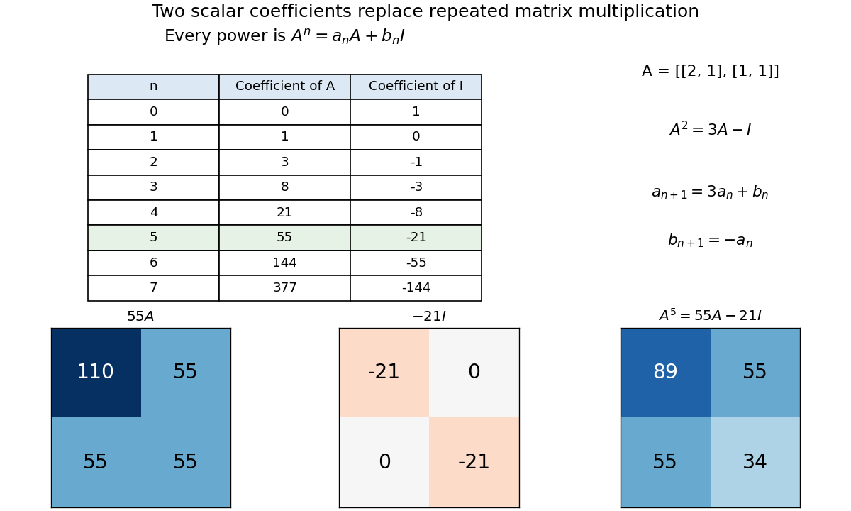
Cayley–Hamilton reduces powers of a chosen two-by-two matrix to two integer coefficients; the fifth power is 55A − 21I
. **Details**.

The same identity computes an inverse. Rearrange it as

A (3 I - A) = I

, giving

A^{- 1} = 3 I - A = (1 - 1 - 1 2) .

(5)

This works because the constant term of this characteristic polynomial is nonzero and the coefficients lie in a field. Generally, when

c_{0} \neq = 0

over a field, rearranging the Cayley-Hamilton theorem expresses

A^{- 1}

as a polynomial evaluated at a matrix. Over a general commutative ring, a nonzero constant need not be a unit; invertibility requires that extra condition.

 Read the full article