Finite-set example of the Johnson–Lindenstrauss lemma

Here is an original reproducible finite set with 40 points and 512 coordinates. Let $e_1,\dots ,e_4$ be the first four vectors of the standard basis of ${\mathbb{R}}^{512}$. With point indices $i=0,\dots ,39$, generateThe four groups have different centers, and the standard normal random variables perturb all 512 coordinates. Generate the coordinates in row order using NumPy's PCG64 pseudorandom number generator with seed 20261013. Then keep this finite set fixed. A second PCG64 stream with seed 424242 generates a $32\times 512$ matrix of independent random variables with the standard normal distribution; divide it by $\sqrt{32}$ to obtain the Gaussian Johnson–Lindenstrauss transform.

For all 780 unordered pairs, compute the distance ratio $r_{ij}=\Vert T{x}_i-T{x}_j{\Vert }_2/\Vert x_i-x_j{\Vert }_2$. In this draw, its minimum is approximately $0.733010$ and its maximum $1.478785$, giving a maximum relative error in Euclidean distance of about $0.478785$. The squared-distance ratios $r_{ij}^2$ instead range from approximately $0.537304$ to $2.186806$: their maximum relative error is about $1.186806$. Thus this particular draw fails a 20% distance tolerance. The Johnson–Lindenstrauss lemma does not assert that every draw into 32 dimensions must succeed.

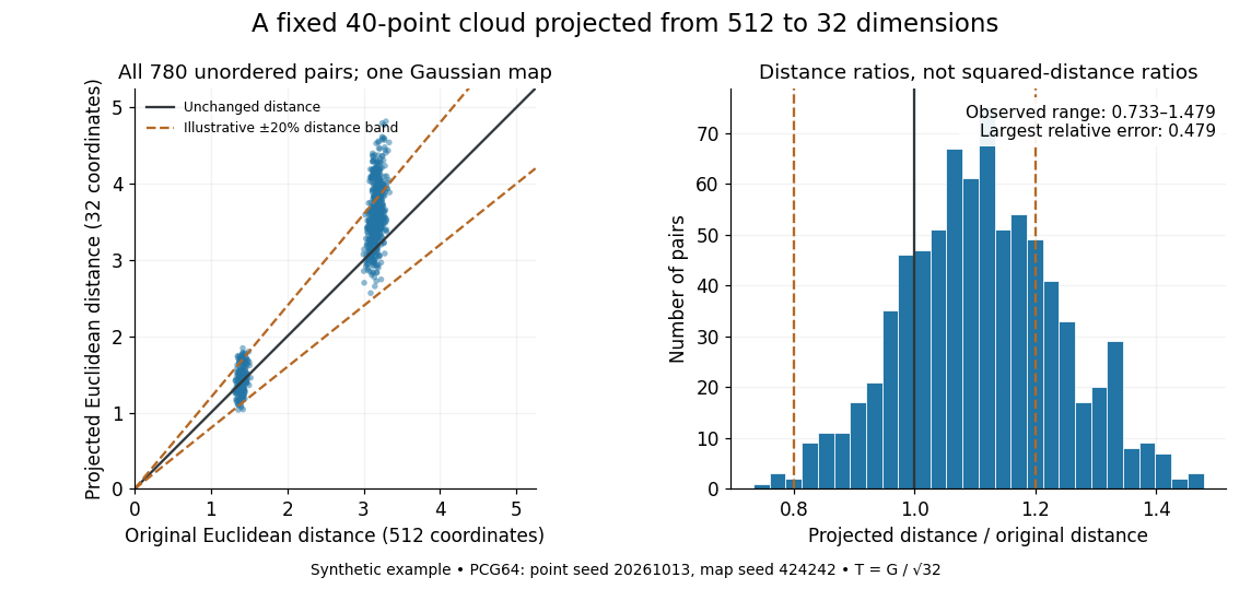
The two bands of original Euclidean distances distinguish pairs within a group from pairs between groups. Their spread after the linear map shows why checking an average distance is insufficient: the Johnson–Lindenstrauss lemma controls every pair. The dashed 20% distance band is an illustrative tolerance, not a confidence interval or a squared-distance band. The affine hull of 40 points has dimension at most 39; 512 is the ambient coordinate count, and no full-dimensionality assumption is required. For this draw the bi-Lipschitz distortion is approximately $1.478785/0.733010=2.017414$.

Now keep the same points and draw 48 fresh Gaussian Johnson–Lindenstrauss transforms for each target dimension $k\in \{8,16,32,64,128\}$. NumPy's SeedSequence(314159).spawn(240) supplies distinct PCG64 streams, ordered first by target dimension, then by draw. Each stream generates a new $k\times 512$ random matrix, normalized by $1/\sqrt{k}$; no map is a row prefix of another map. Each plotted value is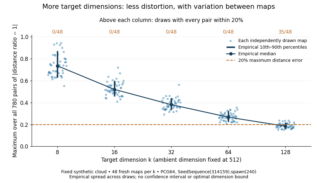

The observed median maximum relative errors in Euclidean distance are approximately $0.735$, $0.520$, $0.381$, $0.267$, and $0.184$, respectively. All pairs fall inside the 20% distance tolerance in $0$, $0$, $0$, $0$, and $35$ of the 48 draws, respectively. These are computations on one synthetic finite set, rather than optimal dimension bounds or measured physical data. The displayed quantiles describe the sampled maps; they do not certify a success probability for other sets. Even at 128 dimensions, 13 of the sampled maps fail this tolerance.

The practical benefit is that each point acquires fewer coordinates while its pairwise Euclidean distances can remain useful. The choice of target dimension balances compression, accuracy, and failure probability. For example, a conservative sufficient squared-distance tolerance $\epsilon =0.2$ with $n=40$ and $\delta =0.05$ gives $k\ge 1195$ by the explicit bound above. Here that exceeds the ambient dimension, so the identity map is better for a certified guarantee. The much smaller dimensions in the plots illustrate observed behavior without claiming that this sufficient bound is sharp.