A metric embedding represents the points of one metric space inside another by an injective function . The geometric question is how faithfully the representation preserves pairwise distances. For example, binary strings can be treated as vectors so that tools from linear algebra become available, but the chosen norm determines what their separation means. A drawing of the points alone does not specify a metric embedding: both metrics matter.
An isometric embedding preserves every distance exactly. A metric embedding that is a bi-Lipschitz map allows multiplicative error while keeping its bi-Lipschitz distortion bounded over all pairs. A coarse embedding instead controls separation through possibly nonlinear functions of distance. These are different requirements: the Hamming cube as an L1 and L2 metric below preserves Hamming distance exactly in one representation and takes its square root in another.
The usefulness is that a complicated distance comparison becomes a calculation with familiar vectors and norms. This also helps assess a visualization: nearby points should not acquire arbitrarily large separations, and far-apart points should not collapse together. Matoušek's 2013 lecture notes describe how motivations from computer science, especially approximation algorithms, accelerated the study of metric embeddings from the 1990s onward. [ref]
Lecture notes on metric embeddings by Jiří Matoušek. Jiří Matoušek, Lecture notes on metric embeddings, preface and Section 1.1
For an injective function between metric spaces with at least two source points, consider all distance ratiosIf constants satisfythen is a bi-Lipschitz map: both and its inverse on are Lipschitz maps. The bound compares the most expanded pair with the most contracted pair. To define the bi-Lipschitz distortion of this particular metric embedding, use the sharp bounds and :Here the Lipschitz constant of is . If no positive finite bounds exist, the bi-Lipschitz distortion is infinite. For a finite source, every injective function has finite bi-Lipschitz distortion, but its size can depend on the source. Matoušek gives the equivalent definition using one scale factor and a multiplicative error bound. [ref]
Lecture notes on metric embeddings by Jiří Matoušek. Matoušek, Section 1.1: distortion and Lipschitz maps
Changing units is harmless: replacing by , with , multiplies both and by and leaves unchanged. In a normed vector space this can be achieved by multiplying every output vector by . Thus bi-Lipschitz distortion one means that all distances change by the same factor; an isometric embedding additionally requires that factor to be one. A stretch factor with a specified normalization is a related quantity; when comparing sources, check which overall scale has been fixed.
Take the four corners , , , of a square, with Euclidean distance in both source and target. For the linear map , the six unordered pairs exhaust the possibilities: the two vertical sides have ratio , the two horizontal sides have ratio , and the two diagonals have ratio . Consequently , , and . In contrast, , three times the identity function, gives ratio for every pair and has bi-Lipschitz distortion .
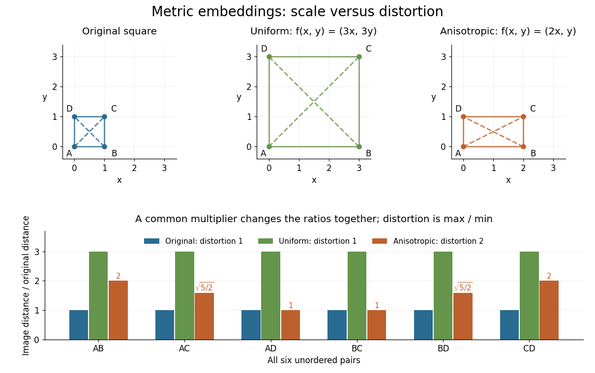
Uniform scaling keeps distortion one; unequal coordinate scaling gives distortion two
. Details. The ratio chart makes the reason visible: a common multiplier moves every ratio together, while unequal coordinate scaling spreads the ratios apart. More generally, in a normed vector space, the ratio bounds giveThis normalization gives Lipschitz constant one and inverse Lipschitz constant . It is only a change of scale, so it cannot improve the bi-Lipschitz distortion.
The best possible bi-Lipschitz distortion of a source into a specified target is a separate quantity:The infimum runs over all injective functions, and need not be attained. The notation means the analogous infimum over metric embeddings into an Lp space. A calculation for one chosen gives an upper bound for ; proving optimality also requires a lower bound for every possible .
For an injective function that does not increase distances, one stretch-factor convention measures the largest compression that must be undone:If the sharp Lipschitz constant of is one, this equals bi-Lipschitz distortion. Fixing the scale matters: uniform compression has stretch factor two in this convention, but bi-Lipschitz distortion one. In a geometric spanner, the corresponding stretch factor is the largest graph-route distance divided by direct Euclidean distance; the graph-to-Euclidean identification does not increase distances. [ref]
https://people.scs.carleton.ca/~michiel/encyc_geometric_spanners.pdf. Gudmundsson, Narasimhan and Smid, Geometric Spanners, §1: the stretch-factor convention
.A map between metric spaces is a coarse embedding when nondecreasing control functions satisfyThe last condition means that distances tending to infinity in the source must also tend to infinity in the target. The upper control prevents bounded source distances from having unbounded image distances. Unlike a metric embedding as defined here, a coarse embedding need not be injective: its lower control may vanish at small distances. Finite bi-Lipschitz distortion implies a coarse embedding by taking and , but nonlinear controls such as allow much more compression.
A family uniformly coarsely embeds into when maps admit the same two control functions and from the definition of a coarse embedding, independent of . For a single finite metric space, the lower control can vanish up to its diameter and then grow without bound; this says little about its representation. For a family with unbounded diameters, common controls have real content: they cannot be chosen afresh after seeing each member's diameter. The Hamming cube as an L1 and L2 metric supplies explicit common controls, in contrast with the expander graph obstruction to uniform coarse embedding.
Use the convention for the Hamming cube . Its elements are length- binary strings, and their Hamming distance counts the differing coordinates:Send each binary string to the vector with the same coordinates, by . Every differing coordinate contributes both to the sum of absolute differences and to the sum of squared differences. Therefore the L1 norm and L2 norm give, respectively,This short coordinate calculation proves that the L1 norm gives an isometric embedding, while Euclidean distance grows like the square root of the number of changed binary digits. For example, and differ twice: their Hamming distance and Manhattan distance are , but their Euclidean distance is . Comparing binary strings in these two geometric representations answers different questions even though the points have the same coordinates.
For distinct pairs ranges over every integer from to . The metric embedding into the L2 norm thus has sharp ratiosNeighbors attain and opposite corners attain . This computes the bi-Lipschitz distortion of this coordinate map; it does not prove that every metric embedding into an L2 space has at least this bi-Lipschitz distortion. Uniformly multiplying the output coordinates changes and together and leaves unchanged.
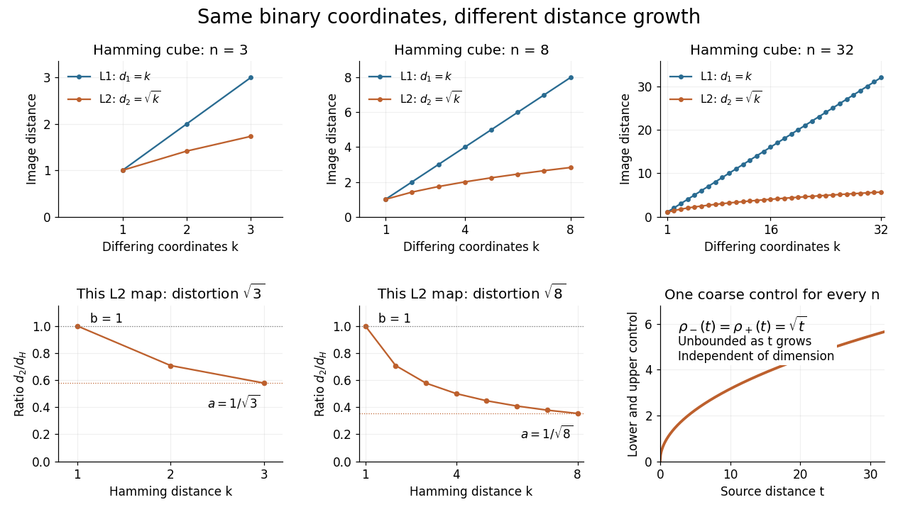
The important family distinction is that these coordinate maps have no dimension-independent bound on their bi-Lipschitz distortion into the L2 norm, yet they do give a uniform coarse embedding of a family of metric spaces. Pad each output vector with zero coordinates to view all maps in the single l2 sequence space, an L2 space for counting measure. Then the same functionswork for every , and . Similarly, padding into the l1 sequence space gives common controls and exact preservation of Hamming distance. These claims use unnormalized Hamming distance; replacing it by normalized Hamming distance changes the family of source metrics.
The geometry has a practical origin: Hamming's 1950 paper uses the number of differing positions between binary strings to study error-correcting codes. Changing one binary digit moves to a neighboring corner, so a question about corrupted messages becomes a question about separation in the Hamming cube. [ref]
https://ineffectivetheory.com/edu/papers/hamming-codes-1950.pdf. R. W. Hamming, Error Detecting and Error Correcting Codes, 1950, Section 5
For a finite graph , its edge-expansion constant isAn expander family has uniformly bounded degrees, orders tending to infinity, and expansion constants bounded below by a positive constant.
For a port-labeled -regular graph and a -regular graph on its port labels, replace every vertex by a copy of . An edge makes a step in , crosses the corresponding edge of , then makes another step in . The result has vertices and degree . Its normalized operator is , where and is the involutive edge rotation of . Decomposing a mean-zero vector into cloud-constant and cloud-orthogonal parts proves the bound .
Choose and a fixed -regular graph on vertices with absolute nonconstant eigenvalues at most . Start with the loop-inclusive complete graph on vertices and iterate . The degree stays , vertex counts are , and . Since , all . The spectral cut bound gives multiplicity-counted edge expansion at least . Removing loops and merging parallel edges loses at most a factor , producing simple expander graphs with maximum degree and edge expansion at least .
If has adjacency matrix and expansion , then every -valued map on its vertices satisfiesFor scalar functions this follows from the layer-cake formula applied above and below a median; integration over the coordinate proves the vector-valued form.
For a nonnegative measurable function ,On a graph, applying this identity to expresses its total variation as the integral of the edge boundaries of the superlevel sets.
More generally, if is differentiable, increasing, and satisfies , then Tonelli theorem and the fundamental theorem of calculus give
Let , , and . Assume the displayed tail inequality and finite positive-threshold superlevel measures. First split at to obtain . Layer cake representation and Tonelli theorem imply . Integrating the original inequality against then gives , with . This is the analytic estimate behind the Doob Lp maximal inequality.
If a -regular graph on vertices has expansion , its distortion obeysThe Poincare inequality controls average image distance by edge lengths, while bounded-degree ball growth makes the average graph distance comparable to .
An expander family does not uniformly coarsely embed into or . Uniform upper control bounds every embedded edge, whereas the expander Poincare inequality bounds the average image distance. A fixed proportion of vertex pairs have graph distance tending to infinity, contradicting the lower control. The case also follows from the isometric Gaussian embedding of a Hilbert space into .
A Banach space is finitely representable in when, for every finite-dimensional subspace and every , there are a subspace and an isomorphism with .
A Banach space is superreflexive when every Banach space finitely representable in it is a reflexive Banach space. Equivalently, it admits an equivalent uniformly convex norm, or every one of its ultrapowers is reflexive.
A Banach space is reflexive exactly when, for every and every sequence in , some convex combination of a finite initial segment lies within of a convex combination of the remaining tail. In a reflexive space both convex hulls approximate a common weak cluster point. The converse is the convex-block form of the James reflexivity criterion.
James's theorem says that a Banach space is reflexive exactly when every continuous linear functional attains its supremum on the closed unit ball. Its separation proof also yields the equivalent convex-block criterion: nonreflexivity produces a bounded sequence whose initial and tail convex hulls remain uniformly separated.
For finite-dimensional subspaces and , the principle of local reflexivity gives an almost-isometric map that fixes and preserves the pairings with . It lets finite-dimensional bidual separation data be realized inside .
A Banach space is superreflexive exactly when, for every , some forces every sequence to have two convex combinations, one before and one after a cut, at distance below . Failure produces a nonreflexive ultrapower; finite representability transfers a violating finite sequence back from any nonreflexive space finitely representable in .
A Banach space is superreflexive exactly when the distortions of the finite diamond graphs tend to infinity. A uniformly separated convex-block sequence recursively realizes all branches of with bounded distortion, while uniform convexity forces quantitative collapse across repeated diamonds.
Every metric space with points admits an embedding into a Hilbert space with distortion . The usual random-subset construction gives an embedding into Euclidean dimension .
Fix a point in a metric space . The Fréchet embedding sends to the bounded function in . The triangle inequality bounds each coordinate by and gives . Taking gives equality, so the map is an isometric embedding. For a separable metric space a countable dense set of anchors suffices. Finite collections of distances to selected subsets instead give one-Lipschitz coordinates that need not be an exact Fréchet embedding.
For every integer , every -point metric space embeds into with distortion at most andThe coordinates are distance-to-subset functions. Randomly sampled subsets at density scales separate every pair at one scale; a union bound leaves the stated number of coordinates.
If a fixed-degree expander on vertices embeds into with distortion , thenIndeed, has distortion , while . Taking gives .
For and any points in a Hilbert space, there is a linear map into Euclidean dimension that multiplies every pairwise distance by a factor between and .
The striking feature is that the target dimension depends on the number of points and the allowed error, independently of the ambient dimension. Fix a finite set , with , and . An equivalent sufficient statement uses squared Euclidean distances: a linear map exists, with , such thatThe finite-set theorem cited here supplies an explicit sufficient target dimension for this squared-distance formulation. [ref]
An elementary proof of a theorem of Johnson and Lindenstrauss by Sanjoy Dasgupta and Anupam Gupta. An elementary proof of a theorem of Johnson and Lindenstrauss, Theorem 2.1, p. 61: bounds for squared distances
Taking square roots gives distance factors and , which lie inside . Conversely, bounds on distances only give squared-distance bounds ; the same numerical tolerance should not be silently used for both. Under the squared-distance bounds, the bi-Lipschitz distortion is at most .
The Johnson–Lindenstrauss lemma preserves this fixed finite set, rather than every vector in the ambient Euclidean space. A linear map with has a nonzero kernel by the rank-nullity theorem, so some nonzero vectors collapse completely. For finitely many points in a real Hilbert space, apply the finite-dimensional argument on their linear span and extend by orthogonal projection onto that linear span. If the sufficient target dimension exceeds the ambient dimension, the identity map already preserves every Euclidean distance exactly, with zero padding if a larger target is requested.
Draw a random matrix whose entries are independent random variables with the standard normal distribution, and setThe factor makes the expected value of the squared L2 norm equal to the original squared L2 norm. This Gaussian Johnson–Lindenstrauss transform is a linear map, generally not an orthogonal projection: its rows are not required to be orthogonal vectors. [ref]
Lecture notes on metric embeddings by Jiří Matoušek. Lecture notes on metric embeddings, §2.1(b), p. 21, and Lemma 2.3.1, p. 24: independent Gaussian coefficients and normalization
For the fixed finite set , let be an allowed failure probability, and defineWith denoting the natural logarithm, a sufficient integer target dimension isThen one draw of this specified random matrix satisfies all the squared Euclidean distance bounds simultaneously with probability at least . Since , the simpler sufficient bound also works. Both are sufficient bounds for this argument; they do not claim the smallest possible target dimension.
This is a probability statement about a map drawn independently of the fixed finite set. It implies existence because the success probability is positive, but permits failed draws. The set cannot be chosen after inspecting the map with this same guarantee. In particular, no single draw preserves every possible finite set in the ambient Euclidean space when .
Here is an original reproducible finite set with 40 points and 512 coordinates. Let be the first four vectors of the standard basis of . With point indices , generateThe four groups have different centers, and the standard normal random variables perturb all 512 coordinates. Generate the coordinates in row order using NumPy's PCG64 pseudorandom number generator with seed 20261013. Then keep this finite set fixed. A second PCG64 stream with seed 424242 generates a matrix of independent random variables with the standard normal distribution; divide it by to obtain the Gaussian Johnson–Lindenstrauss transform.
For all 780 unordered pairs, compute the distance ratio . In this draw, its minimum is approximately and its maximum , giving a maximum relative error in Euclidean distance of about . The squared-distance ratios instead range from approximately to : their maximum relative error is about . Thus this particular draw fails a 20% distance tolerance. The Johnson–Lindenstrauss lemma does not assert that every draw into 32 dimensions must succeed.
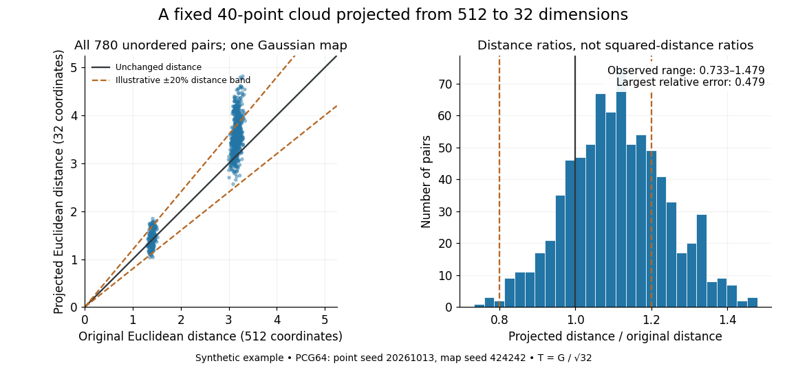
The two bands of original Euclidean distances distinguish pairs within a group from pairs between groups. Their spread after the linear map shows why checking an average distance is insufficient: the Johnson–Lindenstrauss lemma controls every pair. The dashed 20% distance band is an illustrative tolerance, not a confidence interval or a squared-distance band. The affine hull of 40 points has dimension at most 39; 512 is the ambient coordinate count, and no full-dimensionality assumption is required. For this draw the bi-Lipschitz distortion is approximately .
Now keep the same points and draw 48 fresh Gaussian Johnson–Lindenstrauss transforms for each target dimension . NumPy's
SeedSequence(314159).spawn(240) supplies distinct PCG64 streams, ordered first by target dimension, then by draw. Each stream generates a new random matrix, normalized by ; no map is a row prefix of another map. Each plotted value is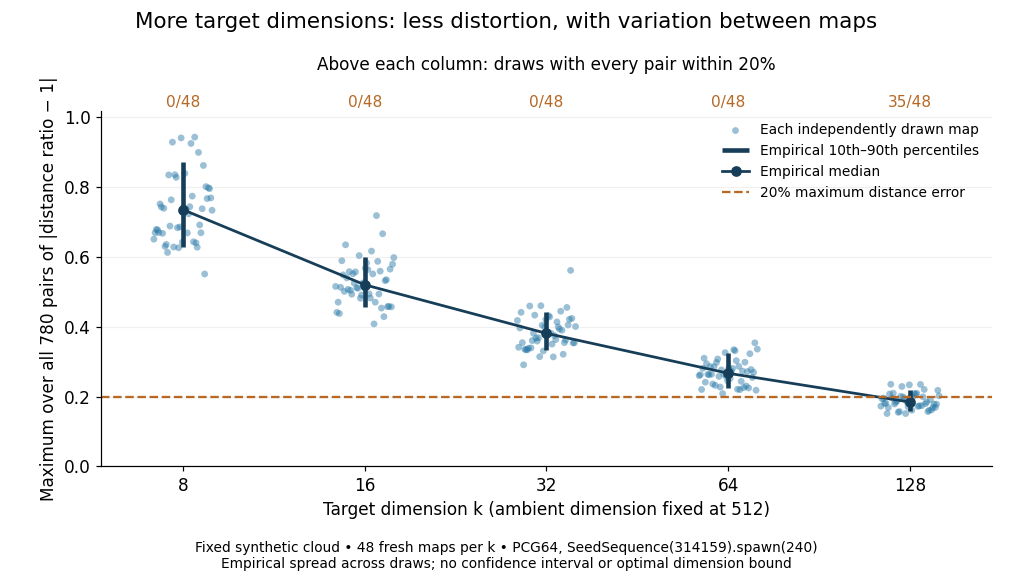


The observed median maximum relative errors in Euclidean distance are approximately , , , , and , respectively. All pairs fall inside the 20% distance tolerance in , , , , and of the 48 draws, respectively. These are computations on one synthetic finite set, rather than optimal dimension bounds or measured physical data. The displayed quantiles describe the sampled maps; they do not certify a success probability for other sets. Even at 128 dimensions, 13 of the sampled maps fail this tolerance.
The practical benefit is that each point acquires fewer coordinates while its pairwise Euclidean distances can remain useful. The choice of target dimension balances compression, accuracy, and failure probability. For example, a conservative sufficient squared-distance tolerance with and gives by the explicit bound above. Here that exceeds the ambient dimension, so the identity map is better for a certified guarantee. The much smaller dimensions in the plots illustrate observed behavior without claiming that this sufficient bound is sharp.
A short concentration inequality argument explains the bound. For a fixed nonzero vector , the normalized row products are independent random variables with the standard normal distribution, soUse the moment-generating function of a chi-squared distribution and the Chernoff bound to obtainFor , elementary logarithm inequalities bound their sum by . Apply the union bound to the nonzero pair differences to get failure probability at most . Independence of different pairs is unnecessary; they use the same map. This combines fixed-vector concentration with a finite-set union bound. [ref]
Lecture notes on metric embeddings by Jiří Matoušek. Lecture notes on metric embeddings, §2.1, pp. 20–21, and proof of Lemma 2.3.1, pp. 25–26: fixed-vector concentration and union bound over pair differences
The unit sphere of an -dimensional normed space has a -net of size at most . If on this net and , then
If has independent Rademacher entries, then for fixed and ,Applying a union bound to all pairwise differences embeds fixed points into dimension while preserving every squared distance within a factor with probability at least .
For a standard normal variable and ,The exponential Markov inequality consequently gives Gaussian concentration for averages of independent copies of .
The random matrixsatisfiesA net argument shows that permits a linear embedding of distortion below .
Every -point metric space embeds into with distortion . Apply the Bourgain embedding theorem, reduce its Euclidean dimension to with the Johnson–Lindenstrauss lemma, and use an Almost-isometric Gaussian embedding from l2 into l1.
Articles by others on the same topic
There are currently no matching articles.