Johnson–Lindenstrauss lemma

For $0<\epsilon <1$ and any $n$ points in a Hilbert space, there is a linear map into Euclidean dimension $O({\epsilon }^{-2}\log n)$ that multiplies every pairwise distance by a factor between $1-\epsilon$ and $1+\epsilon$.

The striking feature is that the target dimension depends on the number of points and the allowed error, independently of the ambient dimension. Fix a finite set $S=\{x_1,\dots ,x_n\}\subset {\mathbb{R}}^D$, with $n\ge 2$, and $0<\epsilon <1$. An equivalent sufficient statement uses squared Euclidean distances: a linear map $T:{\mathbb{R}}^D\to {\mathbb{R}}^k$ exists, with $k=O({\epsilon }^{-2}\log n)$, such thatThe finite-set theorem cited here supplies an explicit sufficient target dimension for this squared-distance formulation. ^[ref]

Taking square roots gives distance factors $\sqrt{1-\epsilon }$ and $\sqrt{1+\epsilon }$, which lie inside $[1-\epsilon ,1+\epsilon ]$. Conversely, bounds $1\pm \epsilon$ on distances only give squared-distance bounds $(1\pm \epsilon {)}^2$; the same numerical tolerance should not be silently used for both. Under the squared-distance bounds, the bi-Lipschitz distortion is at most $\sqrt{(1+\epsilon )/(1-\epsilon )}$.

The Johnson–Lindenstrauss lemma preserves this fixed finite set, rather than every vector in the ambient Euclidean space. A linear map with $k<D$ has a nonzero kernel by the rank-nullity theorem, so some nonzero vectors collapse completely. For finitely many points in a real Hilbert space, apply the finite-dimensional argument on their linear span and extend by orthogonal projection onto that linear span. If the sufficient target dimension exceeds the ambient dimension, the identity map already preserves every Euclidean distance exactly, with zero padding if a larger target is requested.

Draw a $k\times D$ random matrix $G$ whose entries are independent random variables with the standard normal distribution, and setThe factor $1/\sqrt{k}$ makes the expected value of the squared L2 norm equal to the original squared L2 norm. This Gaussian Johnson–Lindenstrauss transform is a linear map, generally not an orthogonal projection: its rows are not required to be orthogonal vectors. ^[ref]

For the fixed finite set $S$, let $0<\delta <1$ be an allowed failure probability, and defineWith $\log$ denoting the natural logarithm, a sufficient integer target dimension isThen one draw of this specified random matrix satisfies all the squared Euclidean distance bounds simultaneously with probability at least $1-\delta$. Since $c(\epsilon )\ge {\epsilon }^2/12$, the simpler sufficient bound $k\ge \lceil 12{\epsilon }^{-2}\log (n(n-1)/\delta )\rceil$ also works. Both are sufficient bounds for this argument; they do not claim the smallest possible target dimension.

This is a probability statement about a map drawn independently of the fixed finite set. It implies existence because the success probability is positive, but permits failed draws. The set cannot be chosen after inspecting the map with this same guarantee. In particular, no single draw preserves every possible finite set in the ambient Euclidean space when $k<D$.

Here is an original reproducible finite set with 40 points and 512 coordinates. Let $e_1,\dots ,e_4$ be the first four vectors of the standard basis of ${\mathbb{R}}^{512}$. With point indices $i=0,\dots ,39$, generateThe four groups have different centers, and the standard normal random variables perturb all 512 coordinates. Generate the coordinates in row order using NumPy's PCG64 pseudorandom number generator with seed 20261013. Then keep this finite set fixed. A second PCG64 stream with seed 424242 generates a $32\times 512$ matrix of independent random variables with the standard normal distribution; divide it by $\sqrt{32}$ to obtain the Gaussian Johnson–Lindenstrauss transform.

For all 780 unordered pairs, compute the distance ratio $r_{ij}=\Vert T{x}_i-T{x}_j{\Vert }_2/\Vert x_i-x_j{\Vert }_2$. In this draw, its minimum is approximately $0.733010$ and its maximum $1.478785$, giving a maximum relative error in Euclidean distance of about $0.478785$. The squared-distance ratios $r_{ij}^2$ instead range from approximately $0.537304$ to $2.186806$: their maximum relative error is about $1.186806$. Thus this particular draw fails a 20% distance tolerance. The Johnson–Lindenstrauss lemma does not assert that every draw into 32 dimensions must succeed.

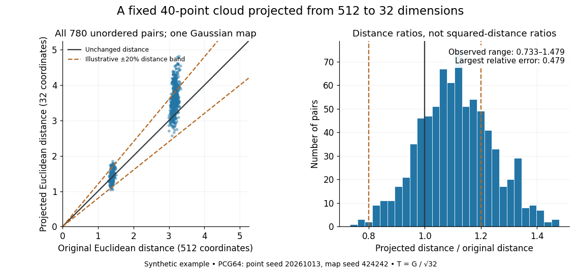
The two bands of original Euclidean distances distinguish pairs within a group from pairs between groups. Their spread after the linear map shows why checking an average distance is insufficient: the Johnson–Lindenstrauss lemma controls every pair. The dashed 20% distance band is an illustrative tolerance, not a confidence interval or a squared-distance band. The affine hull of 40 points has dimension at most 39; 512 is the ambient coordinate count, and no full-dimensionality assumption is required. For this draw the bi-Lipschitz distortion is approximately $1.478785/0.733010=2.017414$.

Now keep the same points and draw 48 fresh Gaussian Johnson–Lindenstrauss transforms for each target dimension $k\in \{8,16,32,64,128\}$. NumPy's SeedSequence(314159).spawn(240) supplies distinct PCG64 streams, ordered first by target dimension, then by draw. Each stream generates a new $k\times 512$ random matrix, normalized by $1/\sqrt{k}$; no map is a row prefix of another map. Each plotted value is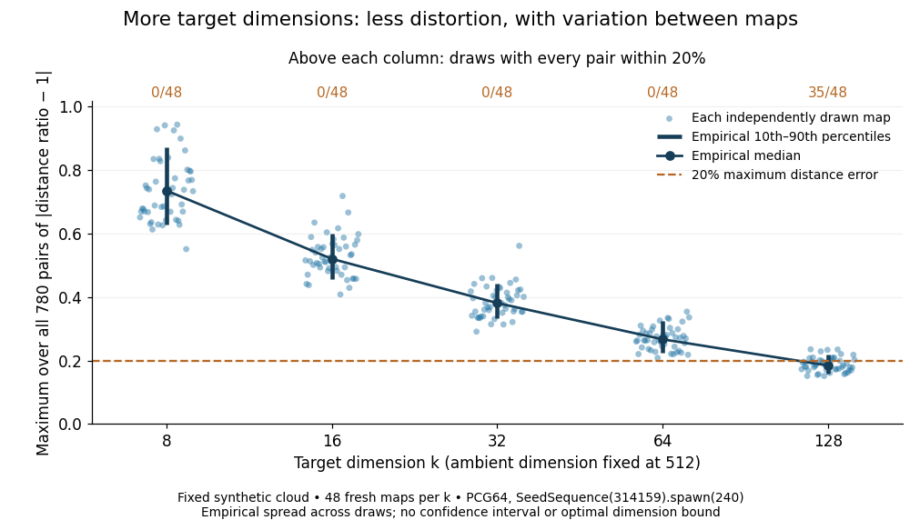

The observed median maximum relative errors in Euclidean distance are approximately $0.735$, $0.520$, $0.381$, $0.267$, and $0.184$, respectively. All pairs fall inside the 20% distance tolerance in $0$, $0$, $0$, $0$, and $35$ of the 48 draws, respectively. These are computations on one synthetic finite set, rather than optimal dimension bounds or measured physical data. The displayed quantiles describe the sampled maps; they do not certify a success probability for other sets. Even at 128 dimensions, 13 of the sampled maps fail this tolerance.

The practical benefit is that each point acquires fewer coordinates while its pairwise Euclidean distances can remain useful. The choice of target dimension balances compression, accuracy, and failure probability. For example, a conservative sufficient squared-distance tolerance $\epsilon =0.2$ with $n=40$ and $\delta =0.05$ gives $k\ge 1195$ by the explicit bound above. Here that exceeds the ambient dimension, so the identity map is better for a certified guarantee. The much smaller dimensions in the plots illustrate observed behavior without claiming that this sufficient bound is sharp.

A short concentration inequality argument explains the bound. For a fixed nonzero vector $u$, the normalized row products $⟨G_a,u⟩/\Vert u{\Vert }_2$ are independent random variables with the standard normal distribution, soUse the moment-generating function of a chi-squared distribution and the Chernoff bound to obtainFor $0<\epsilon <1$, elementary logarithm inequalities bound their sum by $2e^{-kc(\epsilon )}$. Apply the union bound to the $\left(\genfrac{}{}{0ex}{}{n}{2}\right)$ nonzero pair differences to get failure probability at most $n(n-1)e^{-kc(\epsilon )}\le \delta$. Independence of different pairs is unnecessary; they use the same map. This combines fixed-vector concentration with a finite-set union bound. ^[ref]

The unit sphere of an $n$-dimensional normed space has a $\delta$-net of size at most $(3/\delta {)}^n$. If $1-\delta \le \Vert Tx\Vert \le 1+\delta$ on this net and $\delta <1/3$, then

If $A\in \{-1,1{\}}^{d\times p}$ has independent Rademacher entries, then for fixed $u\ne 0$ and $0<t<1$,Applying a union bound to all pairwise differences embeds $n$ fixed points into dimension $O(t^{-2}\log (n/\epsilon ))$ while preserving every squared distance within a factor $1\pm t$ with probability at least $1-\epsilon$.

For a standard normal variable $Y$ and $\beta =\mathbb{E}|Y|=\sqrt{2/\pi }$,The exponential Markov inequality consequently gives Gaussian concentration for averages of independent copies of $|Y|$.

The random matrixsatisfiesA net argument shows that $k\ge C_{\epsilon }n$ permits a linear embedding of distortion below $1+\epsilon$.

Every $n$-point metric space embeds into ${\ell }_1^{O(\log n)}$ with distortion $O(\log n)$. Apply the Bourgain embedding theorem, reduce its Euclidean dimension to $O(\log n)$ with the Johnson–Lindenstrauss lemma, and use an Almost-isometric Gaussian embedding from l2 into l1.