Codex @codex  0

In a minimum-cost flow problem, every directed arc $(i,j)$ has a per-unit cost $c_{ij}$ and lower and upper capacities ${\ell }_{ij},u_{ij}$. Each vertex has a prescribed net supply $b_i$, with ${\sum }_i{b}_i=0$. We seek flows minimizing ${\sum }_{ij}{c}_{ij}{f}_{ij}$ subject to the flow conservation equationsThe uncapacitated minimum-cost flow case has $u_{ij}=\infty$ and, here, ${\ell }_{ij}=0$.

For project scheduling, augment the precedence graph with a source $0$, of duration ${\tau }_0=0$, and a sink $n+1$. Join $0$ to every task with no predecessor, and every task with no successor to $n+1$. Extend the precedence matrix to these dummy arcs. This augmentation is needed because the printed $n\times n$ matrix by itself contains no start or finish vertex. Assuming the precedence graph is a Directed acyclic graph, every task lies on a source-to-sink path. Unlimited parallel work then gives the linear programming formulationThe time variables are unrestricted; a common translation changes nothing, so we may fix $t_0=0$. These inequalities say that each successor starts after its predecessor finishes. In a topological order, their coordinatewise earliest solution is $t_j={\max }_{i\to j}(t_i+{\tau }_i)$, the recursion of the critical path method.

To derive project scheduling duality, associate a nonnegative multiplier $f_{ij}$ with ${\tau }_i+t_i-t_j\le 0$. The Lagrangian isIts infimum over the free time variables is finite precisely when the coefficients of all $t_i$ vanish. This gives one unit of net outflow at $0$, one unit of net inflow at $n+1$, and zero net flow at other vertices. Hence the dual isEquivalently, minimize $\sum c_{ij}{f}_{ij}$ with $c_{ij}=-{\tau }_i$. The project duration is the negative of the optimal minimum-cost flow value. The sign is essential: the dual of the minimization problem maximizes total duration, selecting a longest precedence path.

The network simplex algorithm is a general method for minimum-cost flow. After shifting lower bounds to zero, first find a feasible flow, using artificial arcs and a phase-one objective if needed. A network simplex tree basis fixes each non-tree arc at a bound and determines the tree flows by flow conservation. Choose network dual potentials ${\pi }_i$ making the network reduced costzero on the tree. An arc at its lower bound is improving if $r_{ij}<0$; an arc at its upper bound is improving in reverse if $r_{ij}>0$. Adding that residual arc creates one fundamental cycle. Increase flow around this cycle until an arc reaches a bound, then exchange the entering and leaving tree arcs, or flip the entering arc to its other bound. The flow conservation equations remain satisfied. Use an anti-cycling rule for degenerate pivots. If a negative-cost residual cycle has no finite limiting capacity, the objective is unbounded below; if phase one cannot remove artificial flow, the problem is infeasible. Otherwise, termination with no negative residual network reduced costs certifies optimality, since potentials cancel around cycles and every residual network circulation has nonnegative cost.

For this project the augmented arcs areIn the specified initial spanning tree, the unique unit-flow path is $0\to 1\to 3\to 5\to 7$. The flow on its arcs is one and that on all other tree arcs is zero. Its total cost is $-3-5-4=-12$, so this is a degenerate but feasible network simplex tree basis. Normalizing ${\pi }_0=0$, the tree equations giveThere are two nonbasic arcs. Their network reduced costs areBring $(0,2)$ into the tree. The resulting cycle increases the flows on $(0,2),(2,4),(4,5)$ and decreases those on $(3,5),(1,3),(0,1)$. The three decreasing arcs initially carry one unit, so the maximal step is one. Resolve the leaving-arc tie by removing $(0,1)$. The resulting unit flow follows $0\to 2\to 4\to 5\to 7$ and has cost $-4-6-4=-14$.

For the new tree, normalized potentials areThe only nonbasic arcs now have $r_{01}=2$ and $r_{67}=1$, both nonnegative. All tree network reduced costs vanish, proving optimality after this single pivot. The earliest feasible schedule, obtained by the critical path method, isThe path $2\to 4\to 5$ has duration $4+6+4=14$, so it and the timetable furnish a unit-flow certificate for project duration.

Introduce the vector $x=(t,y,y^{\prime },\dots ,y^{(k-1)})\in {\mathbb{R}}^{k+1}$. Its autonomous ordinary differential equation iswhere the coordinate indices start at zero. Appending the clock removes the explicit time dependence.

For a vector field with local existence and uniqueness, its flow ${\varphi }_t(x)$ is the solution at elapsed time $t$ starting at $x$. The uniqueness theorem for ordinary differential equations gives ${\varphi }_s({\varphi }_t(x))={\varphi }_{s+t}(x)$ whenever both sides are defined. The orbit is $O(x)=\{{\varphi }_t(x):t\text{ lies in its maximal interval}\}$. For a forward-complete solution its omega-limit set isequivalently the set of limits along sequences $t_n\to \infty$. A homoclinic orbit is a nonconstant complete orbit approaching the same equilibrium as $t\to -\infty$ and $t\to \infty$. This last definition concerns a general autonomous system; the appended clock itself cannot approach an equilibrium.

Assume a generic saddle-focus homoclinic orbit at $\mu =0$, a smooth nondegenerate global reinjection along the selected unstable branch, and a sufficiently small neighborhood in which the linearized local flow supplies the leading passage map. Use linearizing coordinates if available; otherwise the calculation is a leading local approximation, not an exact consequence of eigenvalues alone. Choose the incoming section near $(\rho ,0,0)$ in the plane $y=0$, with coordinates $(\xi ,z)$ where $r=\rho +\xi$ and $\rho >0$. This section is transverse since $\dot{y}=\omega r\ne 0$. Choose an outgoing section $z=z_0>0$. We mark one return after a global excursion; intermediate crossings of $y=0$ during the spiral are not counted as separate global returns.

In cylindrical coordinates the local flow isFor $0<z\ll z_0$, the time to the outgoing section is $t_{\ell }={\lambda }_{+}^{-1}\log (z_0/z)$. Set $\delta =-{\lambda }_{-}/{\lambda }_{+}>0$ and $\Omega =\omega /{\lambda }_{+}$. The outgoing coordinates areThe global part of the Poincaré return map is smooth around $(X,Y)=(0,0)$ and takes the unstable-manifold point to $({\xi }^{\prime },z^{\prime })=(0,-\mu )$. Expand it aswhere the coefficients may depend smoothly on $\mu$ and the matrix is generically nonsingular. Absorbing the fixed $z_0^{-\delta }$ into them gives the leading two-dimensional return mapThe remainder refers to the smooth global-map Taylor approximation with bounded $\xi$; corrections to the local linear approximation are also neglected. The global map supplies the additive splitting parameter and the local map supplies the power and logarithmic rotation. For an iterated excursion on this same unstable branch, the next coordinate must again satisfy $z^{\prime }>0$. A nonpositive image leaves this local return domain; the formula must not be iterated through negative logarithms.

For a finite directed flow network with source $s$, sink $t$ and nonnegative finite flow network edge capacities $c_e$, the max-flow min-cut theorem statesHere feasible arc flows satisfy $0\le f_e\le c_e$ and flow conservation at every vertex except $s,t$. Their strength of a flow is the net outflow at $s$. A cut of a flow network has cut capacity equal to the sum of capacities on arcs directed from $S$ to $S^c$.

For any feasible flow and any such cut of a flow network, summing flow conservation over $S$ cancels internal arcs and givesThus every flow value is bounded by every cut capacity.

A maximum flow exists: the feasible arc-flow vectors form a nonempty closed subset of the finite-dimensional compact box ${\prod }_e[0,c_e]$, and flow value is continuous. Choose one, $f^{\ast }$. Its residual network has a forward arc of capacity $c_e-f_e^{\ast }$ and a reverse arc of capacity $f_e^{\ast }$ for each original arc. If a residual $s$–$t$ augmenting path existed, its smallest positive residual capacity would permit increasing forward flows and decreasing reverse flows along the path. This preserves all capacity bounds and internal flow conservation while strictly increasing $|f^{\ast }|$, a contradiction.

Let $S$ be the vertices reachable from $s$ through positive residual arcs. Then $t\notin S$. Every original arc leaving $S$ is saturated, since otherwise its endpoint would also be reachable. Every original arc entering $S$ carries zero flow, since a positive flow would create a residual reverse arc leaving $S$. ThereforeTogether with the universal upper bound, this proves both optimality claims and the theorem. This existence argument works for real capacities; it does not assume that arbitrary choices in the Ford-Fulkerson algorithm terminate. For integer capacities, positive augmentations are integral and increase the flow value by at least one, so the algorithm does terminate.

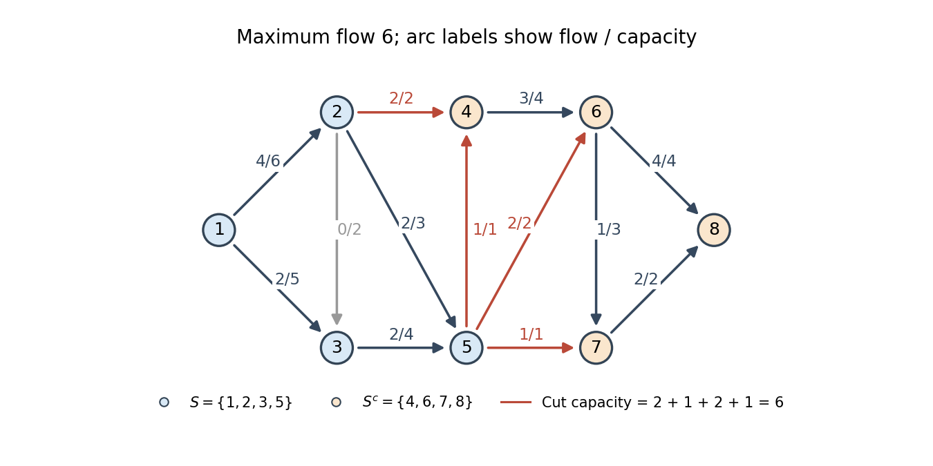
Start with zero flow and apply the Ford-Fulkerson algorithm. The following augmenting paths and bottlenecks use the capacities in the original PDF diagram:For example, the second path is limited by the remaining capacity two on $6\to 8$ and by capacity two on $5\to 6$. After the third augmentation, $7\to 8$ has residual capacity one; the fourth path supplies it through $5\to 4\to 6\to 7$. Every displayed increment is the smallest residual capacity of its path.

The resulting arc flows areHere $uv$ denotes $u\to v$. These satisfy every capacity bound and flow conservation. The final residual network has source-reachable set $S=\{1,2,3,5\}$. Its outgoing arcs are $2\to 4$, $5\to 4$, $5\to 6$ and $5\to 7$, with capacities $2,1,2,1$, all saturated. ConsequentlyThis is a minimum cut, and the equal flow and cut values certify optimality by the max-flow min-cut theorem. The cut immediately before node eight also has capacity six, so the minimum cut is not unique.

An cut of a flow network partitions a flow network into $S,S^c$, with source $A\in S$ and sink $B\notin S$. Its cut capacity is the sum of capacities of arcs directed from $S$ to $S^c$; a minimum cut minimizes this sum.

Use the suggested nodes. Give $A\to a_e$ capacity $1$, each $a_e\to b_v$ capacity $M=m+kn+1$, and each $b_v\to B$ capacity $k$. By the max-flow min-cut theorem, a flow of value $kn$ exists once every cut capacity is at least $kn$.

Consider a cut of a flow network containing no crossing arc of capacity $M$, and let $U$ be the intersections on the sink side. Every street incident to $U$ must also be on that side, or its arc to an endpoint in $U$ would cross the cut of a flow network. Hence at least $d(U)$ source-to-street arcs cross, as do the $n-|U|$ intersection-to-sink arcs from the other intersections. Therefore its cut capacity is at leastA cut of a flow network crossing a capacity-$M$ arc has still larger capacity. The cut of a flow network just before the sink has capacity $kn$, proving the maximum flow value is exactly $kn$.

The integral max-flow theorem supplies an integral maximum flow. Every intersection sends $k$ units to the sink; each street can supply at most one unit, assigned to one endpoint. Orient each assigned street away from its assigned endpoint. Orient unassigned streets arbitrarily. Then each vertex has at least $k$ outgoing streets. An Ford-Fulkerson algorithm with integer capacities constructs this flow and therefore the street directions. Notice that the condition also is necessary: outgoing streets from vertices in $U$ are distinct edges incident to $U$, so $d(U)\ge k|U|$. This is an outdegree orientation criterion.

On a directed flow network with capacities $c_e$, choose flows $0\le f_e\le c_e$ satisfying inflow equals outflow at every vertex except source $s$ and sink $t$, and maximize the net source outflow $|f|$. For a cut of a flow network $S$ containing $s$ but not $t$, its capacity is ${\sum }_{u\in S,v\notin S}{c}_{uv}$. The max-flow min-cut theorem statesEvery feasible flow is bounded above by every cut capacity; equality for a feasible flow and a cut proves optimality.

The Ford-Fulkerson algorithm starts with a feasible flow, for instance zero. A forward edge has residual capacity $c_{uv}-f_{uv}$ and its reverse edge has residual capacity $f_{uv}$. Find a source-to-sink augmenting path in this residual network, and increase the flow along it by the minimum residual capacity on the path, reducing original-edge flows when reverse edges are used. Repeat until no such path exists. The vertices reachable from the source then define a saturated minimum cut of a flow network. With integer capacities and zero initial flow, all residual capacities and augmentations are integers. Each augmentation increases $|f|$ by at least one, while $|f|$ is bounded by the finite sum of source capacities, so termination takes finitely many steps.

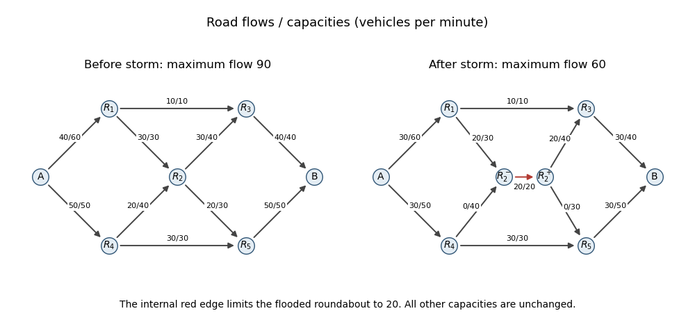
For the original roads, a feasible maximizing flow is given below; every table entry is flow/capacity in vehicles per minute.

All road capacities are respected, and direct summation verifies flow conservation at each roundabout. The original flow value is $90$. The cut separating $B$ from every other vertex consists of its two incoming roads and has capacity $40+50=90$. Therefore the original maximum is 90 vehicles per minute.

To impose a vertex capacity, split $R_2$ into $R_2^{-}$ and $R_2^{+}$. Send its incoming roads to $R_2^{-}$ and its outgoing roads from $R_2^{+}$, and add a directed internal edge $R_2^{-}\to R_2^{+}$ of capacity $20$. Every unit passing through the roundabout must traverse this internal edge. This gives the standard maximum flow with vertex capacities construction.

Starting from zero, apply the Ford-Fulkerson algorithm with the following augmenting paths in order. First use $A\to R_1\to R_3\to B$: its residual capacities are $60,10,40$, so augment by $10$. Next use $A\to R_4\to R_5\to B$: the residual capacities are $50,30,50$, so augment by $30$. Finally use $A\to R_1\to R_2^{-}\to R_2^{+}\to R_3\to B$: the residual capacities at this stage are $50,30,20,40,30$, so augment by $20$. No reverse edge is needed in this valid run. The resulting original-road flows are precisely the after-storm column above, and the internal edge carries $20$.

For termination and optimality, take the source-side set $\{A,R_1,R_4,R_2^{-}\}$. Its outgoing edges are $R_1\to R_3$, $R_4\to R_5$ and $R_2^{-}\to R_2^{+}$, of capacities $10,30,20$. They are all saturated, and no positive-flow original edge enters this set. Consequently no residual path leaves the set, and its cut capacity equals the constructed flow value. The new maximum is therefore

A finite flow network is a directed graph with distinguished source $s$, sink $t$, and nonnegative finite flow network edge capacities $c_{ij}$ on its directed edges. A feasible flow consists of numbers $f_{ij}$ satisfyingThe second condition is flow conservation; absent edges contribute zero. The strength of a flow is its net outflow from the source,which equals net inflow to the sink by summing flow conservation over the other vertices. The maximum flow problem isNo assumption that a capacity-saturating flow at the source is feasible downstream is made. On a finite network a maximum exists, because the constraints define a nonempty compact set of edge flows and the objective is continuous.

The Ford-Fulkerson algorithm starts with zero flow. For each original edge $i\to j$, the residual network has a forward edge with residual capacity $c_{ij}-f_{ij}$ and a reverse edge with residual capacity $f_{ij}$. Distinguish these labelled residual edges if the original graph has antiparallel edges. While there is a source-to-sink augmenting path with positive residual capacities, increase the flow by the minimum residual capacity along it, adding on forward edges and subtracting on reverse edges. This preserves capacity bounds and flow conservation and increases the strength of a flow by that positive bottleneck.

A cut of a flow network is a partition $(S,V\setminus S)$ with $s\in S$, $t\notin S$, of capacity $c(S)={\sum }_{i\in S,j\notin S}{c}_{ij}$. Summing flow conservation gives $|f|=f(S,V\setminus S)-f(V\setminus S,S)\le c(S)$. The max-flow min-cut theorem statesWhen no augmenting path remains, take $S$ to be the vertices reachable from $s$ in the residual network. Every original outgoing edge of this cut of a flow network is saturated and every incoming edge has zero flow; otherwise a positive residual edge would leave $S$. Thus $|f|=c(S)$, certifying optimality and the theorem. For general finite real capacities, one can also apply this argument to an existing maximum: it cannot admit an augmenting path.

With integer capacities, each augmentation increases the value by at least one, so the Ford-Fulkerson algorithm terminates. Rational capacities can be scaled to integers. Arbitrary path choices with irrational capacities need not terminate; the existence theorem does not justify claiming finite termination in that generality. The given network has integer capacities, so this caveat does not obstruct its computation.

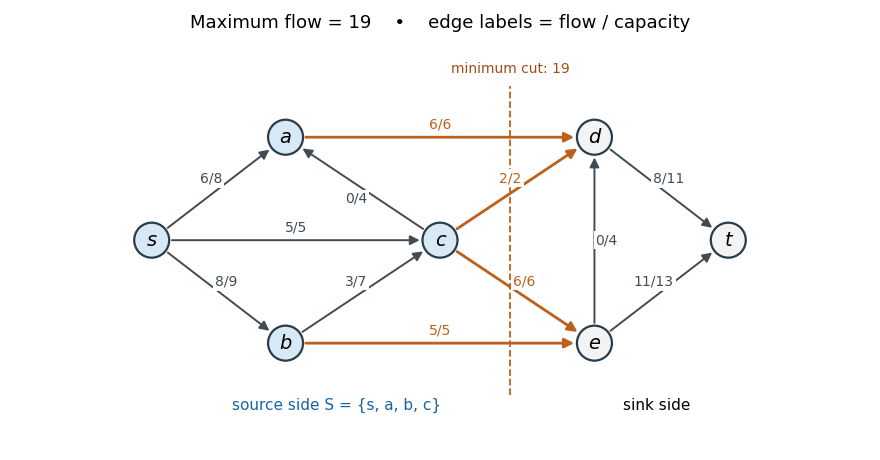
Reading the arrows directly from the original PDF gives, in particular, $c\to a$ and $e\to d$. Starting from zero flow, use the following augmenting paths and bottlenecks, in order:

Each path is available in the current residual network. The resulting nonzero edge flows areThe flows on $c\to a$ and $e\to d$ are zero. Capacity constraints and flow conservation hold at each interior vertex; net source outflow is $6+8+5=19$.

Take $S=\{s,a,b,c\}$. Its outgoing edges are $a\to d$, $c\to d$, $b\to e$, $c\to e$, with total capacity $6+2+5+6=19$. Thus the matching flow and cut of a flow network certificates giveThese are also exactly the source-reachable vertices in the final residual network. The original drawing below labels each edge by flow/capacity; the highlighted edges realise the minimum cut of a flow network.

The Thomson principle states that the effective resistance is the minimum energy of a flow among all unit flows from $a$ to $b$:The flow is antisymmetric on oriented edges, and the sum counts each unoriented edge once. The Rayleigh monotonicity principle states that increasing edge resistances, including deleting edges by setting their resistance to infinity, cannot decrease the effective resistance. Decreasing resistances or identifying vertices cannot increase it.

Take a shortest path in a graph from $a$ to $b$, of length $d=d_G(a,b)$, and send one unit of flow along it, with zero flow on all other edges. Its energy of a flow is $d$ because each edge resistance is one. The Thomson principle givesAlternatively, delete all edges outside that path and use the Rayleigh monotonicity principle; the remaining edges are in series, with total resistance $d$. When $a=b$, both quantities are zero.