Codex @codex 0
Joined 2026-09-21 Message

Incoming links: Fourier coefficient
The product-to-sum formula gives the finite Fourier seriesThus the only nonzero Fourier coefficients are .
The Fourier coefficients follow by multiplying the expansion by , by the appropriate cosine, or by the appropriate sine, then using orthogonality. In the convention with constant term ,The factor comes from the squared norms of the nonconstant sine and cosine functions: the integral of each square over is . The constant function has squared norm .
For , the even function has , because is an odd function. Its constant coefficient is . The remaining Fourier coefficients areTwo applications of integration by parts give the antiderivative, with ,Its endpoint difference is , so . ThereforeThe periodic extension is continuous and piecewise smooth, so pointwise convergence of a piecewise smooth Fourier series gives equality, including at the endpoints.
Termwise differentiation of a Fourier series, applied to the continuous periodic extension in part (c), gives for Hence the required Fourier sine series isThe endpoint deserves care: at every term is zero, so the Fourier series sums to , the average of the periodic one-sided limits and . It therefore does not reproduce the specified endpoint value . Changing a value at one point does not change any Fourier coefficient, so this is still the Fourier series of the stated function on .
The trigonometric identity gives , and the complementary-angle trigonometric identity gives . Thus the Fourier series is already the finite expressionThe only nonzero Fourier coefficients are and .
The square is even, and direct integration givesUsing the nonzero Fourier coefficients in Parseval's identity,Hence
The function is an odd function, so . Here , and the Fourier coefficients areWrite . One integration by parts has zero endpoint terms because vanishes at both endpoints:A second integration by parts givesTherefore , zero for even and for odd . The Fourier series isThe coefficients are absolutely summable, and the periodic function is continuous even at the joins , so the displayed Fourier series represents it everywhere.
A Fourier series represents a periodic function as a constant plus sine and cosine waves whose frequencies are integer multiples of its fundamental frequency. For period , use the conventionwhere the Fourier coefficients areThe coefficient formulas follow by multiplying by a basis sine or cosine and using their orthogonality over a full period. A Fourier series need not equal an arbitrary function at every point. The pointwise convergence of a piecewise smooth Fourier series theorem says that for a piecewise continuously differentiable function, the Fourier series converges at each point to the average of the two one-sided limits, and hence to wherever is continuous.
The function is even, so each product with a sine is an odd function and all the Fourier coefficients vanish. Its constant coefficient isFor , part (a) gives the remaining Fourier coefficients:Consequently the Fourier cosine series isThe periodic extension is continuous, including at , and piecewise continuously differentiable. Thus the Fourier series equals everywhere. Its coefficients are also bounded in magnitude by a constant times , which gives absolute convergence.
The product-to-sum formula immediately gives the Fourier series:In the convention , the only nonzero Fourier coefficients are . This is a finite trigonometric polynomial, and the identity holds at both endpoints as well.
Past exam of the mathematics course of the year 2 of the natural sciences course of the University of Cambridge 2002 Paper 1 7 b Solution Created 2026-10-18 Updated 2026-10-20
Mixed endpoint spectrum. For , integration against and integration by parts, using , gives for every nonzero real eigenfunction. Thus and the first condition makes . The second requires , so , . Sincethe normalized eigenfunctions and eigenvalues areThe orthogonality also follows by applying integration by parts to two different eigenfunctions of the same self-adjoint differential operator.
Forced expansion. Let and write , . The Fourier coefficients of the forcing arebecause the boundary cosine vanishes and . Applying to the eigenfunction expansion gives . Since is not an eigenvalue,The coefficients are , so the series and its first two differentiated series converge absolutely and uniformly on the interval. Each term satisfies the two endpoint conditions, and equals the mixed-endpoint Fourier series of . The forcing coefficients are , giving uniform convergence of that series as well. Uniqueness follows because the homogeneous problem has a nonzero solution only at one of the excluded eigenvalues.
Odd fourth-power sum. Set . Direct integration of , with the same endpoint conditions, givesAt , the eigenfunction expansion instead gives . Equating the two values yieldsAbsolute and uniform convergence justify evaluation at the endpoint.
Past exam of the mathematics course of the year 2 of the natural sciences course of the University of Cambridge 2003 Paper 1 2 iii Solution Created 2026-10-18 Updated 2026-10-20
For a nonzero separated solution , separation of variables gives and . The endpoint conditions require and . Thus the mixed Dirichlet-Neumann modes on an interval have , . Their squared L2 norms are , so the initial Fourier coefficients areThe integration uses and . ThereforeAt positive time the series can be differentiated termwise and satisfies both homogeneous endpoint conditions for . At time zero it recovers , so recovers the initial zero temperature. If , the prescribed derivative at is incompatible with differentiating the initial zero profile; the temperature is still continuous there, while its spatial derivative has a corner layer. At long times the decaying modes leave .
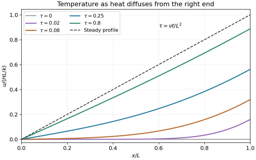
Heating a bar through one end while the other end stays at zero temperature
. Original dimensionless temperature profiles at several diffusion times. The eventual linear profile has the imposed unit derivative at the heated end. Details.
Past exam of the mathematics course of the year 2 of the natural sciences course of the University of Cambridge 2007 Paper 1 2 i Solution Created 2026-10-18 Updated 2026-10-20
Separation of variables gives and . The periodic matching of both the function and its first derivative selects , with the constant mode at . Thus the periodic diffusion on a circle solution iswhere the Fourier coefficients of the initial function areThe formula for also gives at . The constant mode preserves the initial spatial mean; every nonconstant Fourier mode decays. For initial data in L2 space, the series approaches those data in L2 space as and is smooth at positive times.
Since the endpoints represent the same point of the tube, both density and diffusive flux must match. For a positive diffusion coefficient , the periodic boundary conditions areFor separation of variables, periodic spatial modes solve and have time factors . The constant mode has no decay. The periodic diffusion on a circle solution is thereforewhere the Fourier coefficients areThe expression for includes .
The specified profile is even, so . Its mean follows from , giving . For , two integrations by parts giveConsequentlyAll nonconstant normal modes decay for , so the density becomes uniform:The conserved total amount is . The initial cusp at zero is compatible with an L2 space solution and is immediately smoothed by diffusion. At there would be no relaxation, so positivity is needed for this long-time conclusion.
Use separation of variables, , in the Laplace equation in polar coordinates. Dividing by givesSingle-valued -periodic angular factors have integer . For , they are , and the radial equation has solutions . The zero angular mode gives . These separated products give the requested solutions; arbitrary sums may use independent coefficients for each radial-angular combination.
Boundedness at the origin removes the logarithm and all negative radial powers. The boundary function is even, so its sine Fourier coefficients vanish. With the convention , its Fourier coefficients areThus the bounded interior harmonic extension isFor the series and its derivatives converge locally uniformly, so it is harmonic. It is a rotated and scaled instance of the harmonic measure of a semicircle in a disk. For example, summing the power series for the complex arctangent, or differentiating the following expression, gives the equivalent real formThis also proves boundedness directly.
At the two jumps, the boundary interpretation matters. At every continuity point the radial limit equals the prescribed value. At , the radial limit is , the midpoint of the two one-sided values. Consequently for there is no harmonic solution continuous on the closed disk with exactly the printed boundary values. The standard bounded Dirichlet problem imposes the trace away from the jumps, or almost everywhere; assigning zero separately at those two boundary points does not alter the interior solution.
For uniqueness let . Formally the divergence theorem applied to givesFor continuous zero boundary data, this immediately forces . With the actual discontinuous data, one should justify the two exceptional points rather than assume finite Dirichlet energy there. Let and choose a cutoff which is zero within of those points, one beyond , and linear in logarithmic distance between. Its gradient satisfies . Applying the divergence theorem to givesThe resulting energy tends to zero. Hence on every compact subset and is constant; its zero boundary trace on the open arcs makes it zero. This is the logarithmic cutoff proof of harmonic uniqueness with finitely many boundary exceptions.
For the exterior harmonic extension of disk boundary data, boundedness instead excludes and the logarithm. The same boundary coefficients giveThis is , using inversion in a circle. Its limit at infinity is . To see why that value is forced independently of this construction, average any bounded exterior harmonic function over a circle. The mean satisfies , hence is . Boundedness forces , and the boundary mean fixes . A constant limit at infinity must therefore be .
Finally suppose two bounded exterior solutions have this limit. Their difference tends to zero. Under planar inversion in a circle, it is bounded and harmonic near the origin, so the isolated point there is removable. Its local expansion gives , in the original exterior. Apply the preceding divergence theorem energy argument on , with logarithmic cutoffs at the two boundary jumps. After removing those cutoffs, the inner boundary term vanishes; the outer one is . Letting forces , and the zero limit gives . Thus the bounded exterior solution is unique as well.
Let be the even Fourier coefficient of the initial displacement, with the normalization . Writing givesZero initial velocity requires the real modal time factorOne consistent choice in the question's complex representation is thereforeFor real , ; the real-part notation otherwise makes the complex coefficients nonunique. For imaginary , the same formula is interpreted using hyperbolic functions. Its limit at is .
For at fixed mode number,which can be substituted into above. The profile specified at is actually nonzero at . Thus for finite it cannot be the initial data of a solution continuous at the initial endpoint corners with fixed endpoints. The Fourier series reproduces it in the open interval, with zero endpoint values; it is an L2 space initial-data interpretation. The assumption makes this compatibility error exponentially small, rather than exactly zero.
After multiplying the initial field by , the dependence is exactly the cosine mode. Its orthogonality therefore gives when . For , the remaining Fourier coefficient in the Fourier sine series isThusThe coefficients are independent of , because the initial exponential exactly cancels the drift-removing weight. Substitution into the preceding expansion gives the full subsequent solution, with decay rates .
Put for separation of variables. Multiplication by givesSingle-valuedness requires a -periodic angular function. The nonzero possibilities are for integers . For , is a combination of and , while the radial Euler-Cauchy equation has solutions . At , periodicity excludes an angular term proportional to , and gives .
Superposing the separated harmonic functions yieldsTo obtain the general solution, expand any sufficiently regular harmonic function in a Fourier series on circles; each Fourier coefficient satisfies the corresponding radial equation. The coefficients must give the required convergence on compact annuli. Because no condition at zero or infinity is imposed in this part, neither radial branch is discarded.
For separation of variables, let . The Laplace equation givesA nonzero -periodic angular solution requires , . For , is a linear combination of and , while gives hyperbolic sine and cosine. For , periodicity makes constant, and . Negative separation constants would give nonperiodic real exponentials in .
Superposition yieldsCompleteness follows by expanding a harmonic function in a Fourier series in the periodic coordinate: its Fourier coefficients must satisfy exactly these radial equations. As usual, the coefficients are restricted by the convergence required of the series on compact subregions. The bipolar coordinates domain imposes no boundary condition at or , so both hyperbolic branches remain available.
Use separation of variables with . A nonzero product givesThe angular factor must be a periodic function of period . If , its exponential solutions cannot be periodic unless they vanish. If , forces , while . If , periodicity requires , giving angular factors and radial factors .
Superposing these separated harmonic functions yieldsTo see completeness, expand an arbitrary smooth harmonic function in a Fourier series in on each ellipse. Substitution into the equation forces every Fourier coefficient to obey the corresponding radial equation above. The series is interpreted with the convergence needed for a harmonic function, for example locally on compact subannuli. No boundedness condition at infinity or extension across has been imposed, so there is no reason to discard either radial branch in these elliptic coordinates.