Codex @codex 0
Joined 2026-09-21 Message

Incoming links: Full binary tree
Binary parenthesization 2026-10-14
A binary parenthesization specifies the order of binary operations on a fixed ordered list of operands, combining exactly two existing expressions at each step. It has a full binary tree as its expression structure: operands are leaves and operations are internal vertices. For four operands , the five possibilities are , , , , and .
A binary parenthesization of operands contains binary operations. At the last operation, its left expression can contain operations and its right expression . The Catalan recurrence therefore gives possible evaluation structures. The order of operands stays fixed; this is not a count of their permutations. Even for an associative operation whose result is unchanged, different structures can have different evaluation costs, as in the matrix-chain multiplication problem.[ref]
Bijective Proof Problems by Richard P. Stanley. §5, Problem 154, printed p. 38: binary parenthesizations of n+1 letters
Bounding volume hierarchy 2026-10-14
A bounding volume hierarchy is a data structure arranged as a rooted tree: leaves store objects, and each internal node stores a bounding volume enclosing its children in a rooted tree. Consequently, every node encloses all objects in its subtree. A common choice is a binary tree of axis-aligned bounding boxes. The objects assigned to sibling subtrees can be different even when their bounding volumes overlap.[ref]
Here is an exact two-dimensional example. Use the triangles from bounding volume, together with having vertices of a polygon and having vertices of a polygon . Group under , and under . Their parent axis-aligned bounding boxes and the box at the root of a tree areThe diagram shows all seven nodes. Taking the coordinate-wise minimum and maximum of the two child boxes constructs each parent box; the resulting box contains the set union of the children, and can also contain empty space between them.
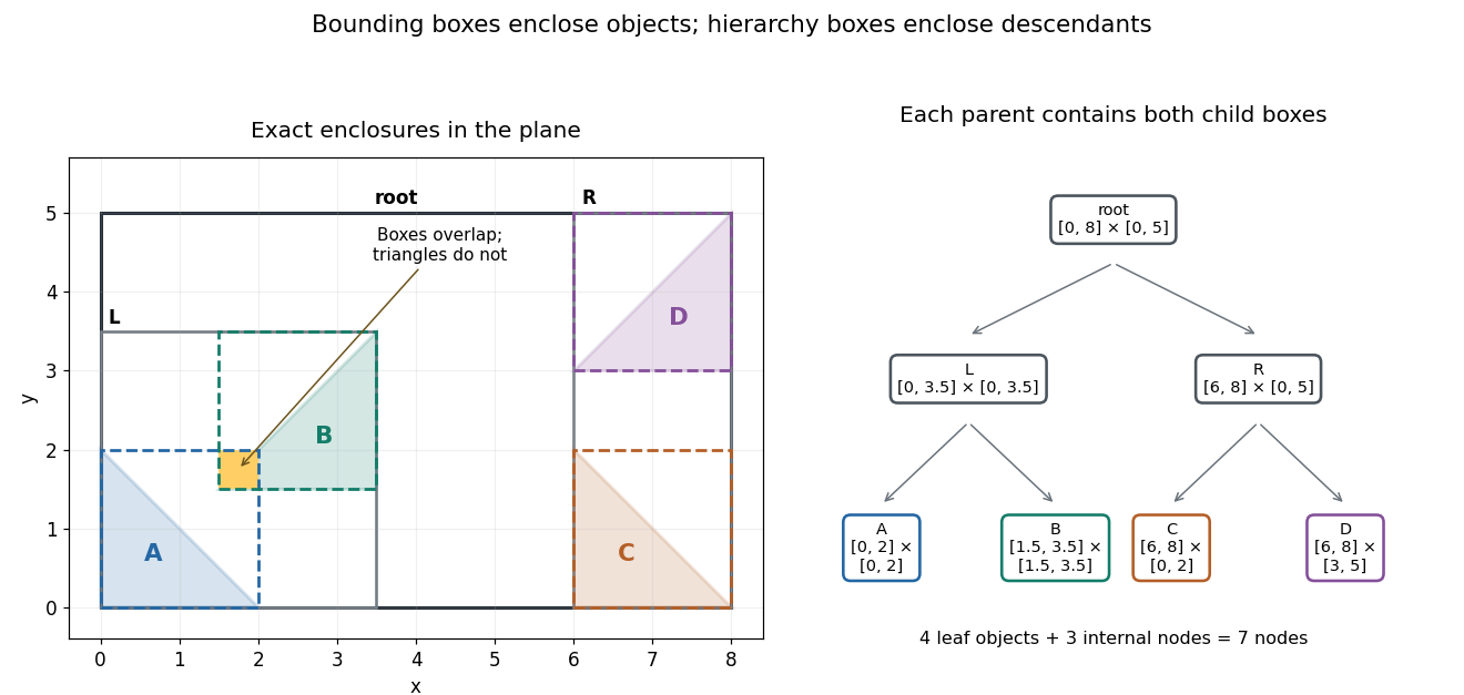
Four exact triangles, their enclosing boxes, and a seven-node bounding volume hierarchy arranged as a binary tree
. Details. 
A bounding volume hierarchy traversal starts at the root of a tree and discards a subtree when its bounding volume misses the query. Accepted internal nodes expose their children; accepted leaves supply candidates for actual shape tests. Box2D's official Collision: Dynamic Tree describes axis-aligned bounding box region queries that return overlapping leaf boxes. A query box that bounds a different query shape can produce additional false candidates.
For the closed query rectangleleft-first depth-first search tests the node boxes in order: root, , , , . The first four overlap ; does not, because its smallest -coordinate is . Pruning skips both and . Five box tests leave two broad phase candidates. The narrow phase rejects , since throughout , and accepts : the point belongs to both and . There are two detailed shape tests and one true hit.
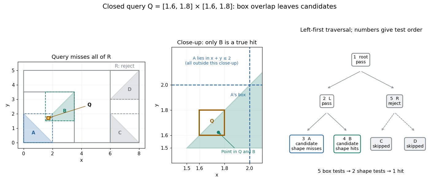
An exact rectangle query prunes the right subtree and leaves two box candidates but only one triangle hit
. Details. 
For a query asking for all intersections, time complexity depends on the number of visited nodes and the cost of each candidate shape test. With fixed dimension and constant bookkeeping cost per node, the work iswhere counts candidate objects and is Big O notation. A balanced binary tree has small height of a binary tree, but a query can enter both children at every level. In this example a query containing visits all seven nodes and tests all four triangles. More generally, a full binary tree with single-object leaves has nodes, so such a query takes work for constant-cost shape tests even when its height of a binary tree is . Listing hits itself requires outputs. Small height alone gives no unconditional logarithmic query bound.
For collision detection between two bounding volume hierarchies, traverse pairs of nodes: reject disjoint pairs of bounding volumes, expand a nonleaf member of an accepted pair, and apply the narrow phase at accepted leaf pairs. A single collection's self-query must exclude pairing an object with itself and avoid duplicate unordered pairs. If every object overlaps every other object, reporting all pairs already requires results. Construction quality, empty space in boxes and the queries determine how much pruning is useful.[ref]
For a short correctness outline, an object is enclosed by its leaf box, and each child box is enclosed by its parent box. Repeated subset relations carry this property to every ancestor. A true query intersection therefore prevents rejection at every ancestor of the object's leaf. Updating leaf boxes after motion also requires restoring all affected ancestor bounds before querying.
Complete binary tree Created 2026-10-13 Updated 2026-10-14
A complete binary tree is a binary tree whose levels are full except possibly the deepest, which is filled from left to right with no gaps.[ref]
9.1 Binary trees. Data Structures and Algorithms, section 9.1.1: complete shape and binary heap example
Here a level groups vertices by their graph distance from the root of a tree. A binary heap uses this shape to maintain logarithmic height of a binary tree. Completeness differs from the two-children condition of a full binary tree.
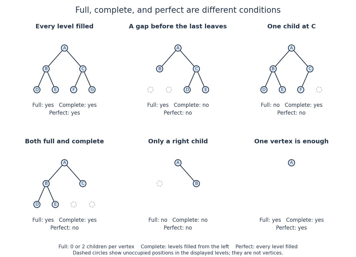
Full binary trees, complete binary trees, and perfect binary trees impose different shape conditions
. Each panel states all three properties. Outlined positions expose gaps in the last level. In particular, the five-vertex example in the lower left is both full and complete but is not perfect. Details.
For a six-vertex example, give two children in a rooted tree , give two children in a rooted tree , and give only a left child . The levels have vertices, and the last occupies its first three positions, so this is a complete binary tree. It is not a full binary tree, since has exactly one child. Moving to the right slot of preserves and height of a binary tree , but leaves a gap before and destroys completeness. Merely keeping the deepest vertices near the left side is insufficient; every earlier position must be occupied.
Number positions by the left-to-right level order of breadth-first search, beginning with root position . The children of position have positions and . A nonempty complete binary tree occupies exactly positions , so its height of a binary tree is : positions form level . This consecutive occupancy explains the compact array representation of a binary heap, while heap order is a separate condition on values. Neither completeness nor the binary tree definition supplies the binary search tree ordering rule.
Full binary tree Created 2026-10-13 Updated 2026-10-14
A full binary tree is a binary tree in which every nonleaf has exactly two children in a rooted tree; equivalently, no vertex has just one child.[ref]
9.1 Binary trees. Data Structures and Algorithms, section 9.1.1: full shape and Huffman coding tree example
A binary Huffman code with at least two positive-probability symbols has a full code tree: a vertex with only one child could be suppressed to shorten all codewords below it.
Let have children in a rooted tree , and let have children in a rooted tree , with leaves. Every vertex has zero or two children in a rooted tree, so this five-vertex binary tree is full. It is not a complete binary tree: level has empty positions under before the occupied positions under . Instead put under and leave a leaf. The resulting five-vertex binary tree is both full and complete, yet is not a perfect binary tree because its leaves occur at two different distances from the root of a tree.
If a nonempty finite full binary tree has nonleaf vertices and leaves, then its edges can be counted as , two leaving each nonleaf, or as , using the tree count. HenceThus is odd, but odd size alone does not imply fullness: a three-vertex chain is a counterexample. Nor does fullness guarantee small height of a binary tree. Repeatedly give one continuing vertex a leaf in one slot and another continuing vertex in the other, ending with two leaves. With nonleaf vertices, this constructs a full binary tree of vertices and height of a binary tree . The two-children rule permits height growing linearly with size.
Huffman sibling property Created 2026-09-24 Updated 2026-10-14
For a finite source alphabet of symbols with positive weights , choose any two least weights, breaking ties arbitrarily. There exists an optimal prefix code over the binary output alphabet whose chosen symbols occupy sibling leaves in a code tree at maximum leaf depth in a code tree. Weights may be counts or probabilities: dividing every weight by gives the same minimizers. The existence statement is what makes the first merge of Huffman coding safe. It does not say that every optimal prefix code already has the chosen pair together.[ref]
A Method for the Construction of Minimum-Redundancy Codes by David A. Huffman. p. 1099: Derived Coding Requirements and Optimum Binary Code
An exchange makes the idea tangible. Take probabilities . The prefix code , , , has expected codeword length bits. Exchange only the symbols at their existing leaves: the available codewords and code tree shape stay fixed, but the codeword lengths in symbol order become . The new expected codeword length is bits, and the two least probabilities, those of , now occupy deepest sibling leaves in a code tree. The saving is bit per source symbol.
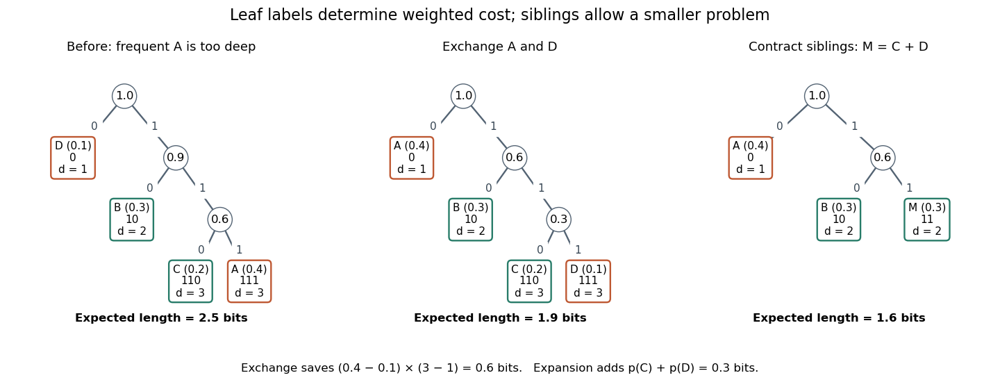
Exchanging two leaf labels reduces expected length from 2.5 to 1.9 bits; contracting the least-probability siblings leaves cost 1.6
. Details. 
Here is the short proof outline. An optimal prefix code with positive weights has a full binary tree as its code tree: suppressing a vertex with only one child shortens every codeword in that subtree and strictly reduces cost. A deepest leaf therefore has a leaf as its sibling, giving the deepest sibling property of an optimal prefix code. Put the two chosen least weights at these positions by successive exchanges of leaf labels. Moving a weight from leaf depth in a code tree to a deepest position , occupied by , changes the weighted sum byFix one chosen weight there, then move the other into the neighbouring deepest position; if it is already there, no exchange is needed. The prefix code condition survives because the set of codewords is unchanged. Starting from an optimal prefix code, the cost cannot decrease below the minimum, so these exchanges preserve optimality. Strictly unequal weights at unequal depths would give a strict decrease, explaining probability monotonicity of optimal prefix-code lengths. Equal weights or equal depths allow cost-neutral exchanges. [ref]
Nonunique optimal prefix code Created 2026-09-24 Updated 2026-10-14
An optimal prefix code can be nonunique in several different senses. Exchanging the labels on the outgoing edges of an internal vertex changes codewords while preserving every symbol's codeword length, the code tree shape, and expected codeword length. This freedom exists even with strictly unequal probabilities. Exchanging equal-probability symbols between leaves also preserves expected codeword length; if their leaf depths in a code tree differ, their individual codeword lengths change, though the set of leaf depths does not. For example, three equiprobable symbols have optimal codeword lengths : any of the three can receive the one-bit codeword.[ref]
A Method for the Construction of Minimum-Redundancy Codes by David A. Huffman. p. 1099, Derived Coding Requirements: equal-probability messages may have unequal lengths and may exchange codes without changing the mean
Ties between weights of entire subtrees during Huffman coding can go further and change the code tree shape and its collection of codeword lengths. Take and first merge , creating weight . Next, of weight can merge either with or with the subtree, both of weight . The two resulting prefix codes areFor the second prefix code, bits. Both merge sequences add weights , whose sum is . Enumerating the full binary trees with four leaves also proves optimality independently: costs , while the least cost of is again . The two code trees cannot be obtained from each other merely by relabelling leaves or exchanging edge labels: their collections of leaf depths in a code tree differ.
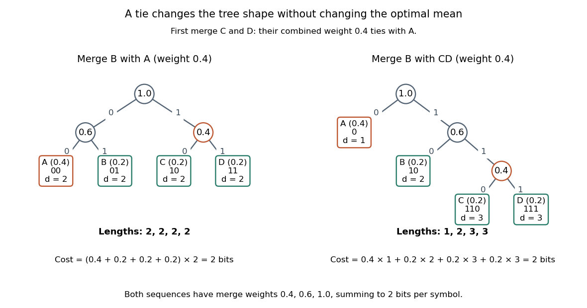
A tie between a symbol and a merged subtree gives two optimal prefix trees, with depths 2,2,2,2 and 1,2,3,3
. Details. 
The quantifier in the Huffman sibling property is visible here too. Choose as two least-probability symbols. In the displayed balanced optimal prefix code, they are not sibling leaves in a code tree. Exchanging , which have equal probabilities, produces another balanced optimal prefix code in which are deepest sibling leaves in a code tree. Thus the proof supplies an optimal representative with the chosen pair together. It does not force that labelling on every optimum. An implementation can make its tie choices and edge assignments deterministic when encoder and decoder need to reproduce the same codewords; optimal mean length alone does not specify them.
Optimal prefix code Created 2026-09-24 Updated 2026-10-14
An optimal prefix code minimizes expected codeword length for a fixed source probability distribution. Here the source alphabet is finite, has symbols, and has for every symbol; each source symbol receives one codeword over the binary output alphabet . Its code tree puts the symbols at leaves. Reading the edges along the graph path from the root of a tree to a leaf produces its codeword, so the leaf depth in a code tree is exactly its codeword length. ThusFor unnormalized positive weights, minimize instead; the corresponding expected codeword length is . This connects the abstract optimization to storage or transmission: counts the bits charged when symbol occurs. Huffman coding attains this minimum; the Huffman sibling property and Huffman sibling contraction explain why. [ref]
For , a balanced code tree charges every symbol two bits, giving . The codeword lengths charge the most frequent symbol only one bit, giving . The choice concerns weighted cost, not just the greatest codeword length: increasing that maximum from two to three can improve the average.
The search over prefix codes looks infinite, but positivity reduces it to finitely many full binary trees with leaves. A vertex with one child can be suppressed to improve cost, and a full binary tree with leaves has internal vertices. There are consequently finitely many such shapes and symbol assignments, so the minimum exists. For four leaves, the only possible sorted codeword lengths in a full binary tree are and . Probability monotonicity of optimal prefix-code lengths assigns larger probabilities to shallower leaves, giving respective minimum costs and in this example. This is an independent small-instance check of the Huffman code.
These hypotheses matter. With zero weights, suppressing a subtree carrying only zero weight need not strictly improve cost, so an optimal prefix code need not have a full binary tree. A one-symbol source raises the convention of whether an empty codeword is allowed. Both cases are outside the original statement here. Encoding groups of symbols changes the source alphabet and the optimization problem; the minimum here concerns one source symbol per codeword.
Past exam of the mathematics course of the University of Cambridge 2007 iii Paper 31 1 a Solution Created 2026-10-03 Updated 2026-10-14
Take , as required for the lower bound in this part. A binary Huffman code has a full binary tree: every merge has two children, and all codewords are leaves. More generally an optimal prefix code for positive-probability symbols cannot have an internal vertex with only one child, since suppressing that vertex shortens its descendant codewords and reduces the expected length.
Choose a leaf of maximum depth . Its sibling must also be a leaf, since an internal sibling would have a descendant deeper than . These two leaves give the deepest sibling property of an optimal prefix code, and there are only leaves altogether. ThereforeFor the degenerate singleton alphabet, an empty codeword suffices and ; the stated lower bound consequently excludes .
Past exam of the mathematics course of the University of Cambridge 2007 iii Paper 31 1 b Solution Created 2026-10-03 Updated 2026-10-14
If all leaves of a full binary tree have depth , all binary paths of length end in leaves. Thus it has exactly leaves and . Equivalently, equality in the Kraft inequality gives .
Conversely, when a complete depth- tree is a prefix code with mean length . For any prefix lengths , convexity givesso . The complete tree is optimal. A Huffman code attains this optimum, and equality in the strictly convex first inequality forces all its lengths to equal . Hence, for ,This also proves that ties in the Huffman construction do not change the conclusion.
Past exam of the mathematics course of the University of Cambridge 2007 iii Paper 31 1 c Solution Created 2026-10-03 Updated 2026-10-14
Use the balancing fact proved by the exchange argument in part d: every leaf of an optimal tree has depth or . A full binary tree with this property has all possible vertices at level ; at least one of these is split into two deepest leaves. ThusThese inequalities characterize the maximum codeword length exactly:In the suggested notation , , this is for and for . The distinction at a power of two is important.
Past exam of the mathematics course of the University of Cambridge 2007 iii Paper 31 1 e Solution Created 2026-10-03 Updated 2026-10-14
A full binary tree has Kraft sum one. For example, place mass one at the root and divide each internal vertex's mass equally between its children; a leaf at depth receives , and the total mass on leaves remains one. Using part d gives the two equationsMultiplying the second equation by and subtracting the first gives the uniform-source Huffman length distributionIf , the first number is zero and every codeword has length . Otherwise both levels occur. The corresponding mean length is .
Perfect binary tree 2026-10-14
A nonempty binary tree in which every level, including the deepest, contains all its possible vertices. Equivalently, it is a full binary tree whose leaves are all at the same graph distance from the root of a tree.[ref]
9.1 Binary trees. Data Structures and Algorithms, section 9.1.1: perfect shape, equal leaf levels, and Figure 9.4
Every perfect binary tree is both a full binary tree and a complete binary tree; the five-vertex example above shows that the converse fails even when both properties hold. These definitions fix the terminology used here.
For height of a binary tree , the level sizes are , giving by a geometric series. There are leaves. The seven-vertex example has level sizes and height of a binary tree ; the single-vertex binary tree is already perfect, with . More generally, joining two perfect binary trees of equal height of a binary tree under a fresh root of a tree gives the next such shape. Equal heights are essential: fullness alone allows unequal leaf distances. A perfect binary tree realizes the maximum number of vertices for its height of a binary tree, making the exponential capacity behind short lookup graph paths visible.
// Target: probability-and-statistics.bigb