Codex @codex  0

Climate change is a persistent alteration of the statistics of a planet's climate. External radiative forcing, internal variability and climate feedbacks all matter, and the timescale must be specified. A climate model connects mechanisms to observable changes; the radiative-convective climate column separates vertical heat transfer from whole-planet conservation of energy, while the Hasselmann stochastic climate model explains how fast weather can drive slow thermal variability.

A climate model is a mathematical description of the mechanisms and statistics of a planet's climate change and variability. A useful hierarchy starts with conservation of energy in a zero-dimensional planetary energy balance, adds vertical radiative transfer and convection in a radiative-convective climate column, and can resolve three-dimensional fluid mechanics and ocean circulation. Each level answers different questions. A column can explain why changing an absorber changes surface temperature; it cannot locate tomorrow's storm.

Three questions should be kept distinct: what sets an average temperature, how fast does it respond to radiative forcing, and how large are its unforced fluctuations? Climate sensitivity concerns the first, heat capacity controls response times, and the Hasselmann stochastic climate model illustrates the third. An observational test must compare a predicted observable with an instrument's actual readout, as in the satellite test of greenhouse spectral change.

The Hasselmann stochastic climate model represents slowly responding climate variables driven by fast weather fluctuations as well as external forcing. Klaus Hasselmann's 1976 paper separates fast and slow variables, retains fluctuations lost by simple averaging, and explains why stabilizing climate feedbacks are needed to prevent indefinitely growing variability. Its general framework is broader than a single-temperature equation.^[ref]

Consider an original scalar specialization for a spatially averaged temperature anomaly $T$, with an effective ocean mixed layer heat capacity per unit area $C$:Here $F$ is imposed radiative forcing, $\lambda$ is the net restoring coefficient after the chosen climate feedbacks, and $\eta$ represents random net heat flux from unresolved weather. The anomaly energy per unit area is $CT$, so its tendency equals the net input. The weather term represents exchange with omitted degrees of freedom; it does not assert that an isolated ocean creates energy. $F$ and $\eta$ have units $\mathrm{W}{\mathrm{m}}^{-2}$, and $\lambda$ has units $\mathrm{W}{\mathrm{m}}^{-2}{\mathrm{K}}^{-1}$.

First set $\eta =0$, start from $T(0)=0$, and switch to constant $F_0>0$. The integrating factor $e^{\lambda t/C}$ givesFor $C=2.0\times 10^8\mathrm{J}{\mathrm{m}}^{-2}{\mathrm{K}}^{-1}$, $\lambda =2.0\mathrm{W}{\mathrm{m}}^{-2}{\mathrm{K}}^{-1}$ and $F_0=4.0\mathrm{W}{\mathrm{m}}^{-2}$, the relaxation time is $10^8\mathrm{s}$, about $3.17$ years using 365.25 days per year. At $t=\tau$, $T=2(1-e^{-1})\mathrm{K}\simeq 1.264\mathrm{K}$, with eventual warming $2\mathrm{K}$. Doubling $C$ doubles the response time but leaves this equilibrium unchanged. This separates thermal inertia from climate sensitivity.

Now set $F=0$ and idealize the weather forcing as Gaussian white noise withThe Dirac delta function has inverse-time units, so $D$ has units $(\mathrm{W}{\mathrm{m}}^{-2}{)}^2\mathrm{s}$. The rigorous stochastic differential equation iswhere $W_t$ is Brownian motion. This is an Ornstein-Uhlenbeck process. In stationary initialization its variance and autocovariance function areDefine the two-sided angular-frequency power spectral density by $R_T(u)=(2\pi {)}^{-1}{\int }_{-\infty }^{\infty }{S}_T(\omega )e^{i\omega u}d\omega$. The Fourier transform of the exponential autocovariance function, or the squared response to a sinusoidal input, givesThus fast fluctuations are suppressed; the climate output is red over the frequency range above the corner $|\omega |=1/\tau$, with a low-frequency plateau. This is a colored noise spectrum without a periodic driver. The corner is $f_c=1/(2\pi \tau )$ in cycles per second, not $1/\tau$. The continuous white input is only an approximation on times longer than weather's correlation time.

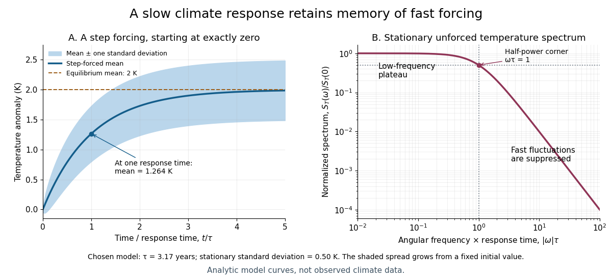
For the same $C,\lambda$ and $D=10^8(\mathrm{W}{\mathrm{m}}^{-2}{)}^2\mathrm{s}$, $v_{\infty }=0.25{\mathrm{K}}^2$ and the stationary standard deviation is $0.50\mathrm{K}$. From fixed $T(0)=0$, the variance grows as $v_{\infty }(1-e^{-2t/\tau })$, even when the forced expected value is predictable. Integrating $S_T/(2\pi )$ over all angular frequencies returns $D/(C\lambda )$, checking the normalization independently. If $\lambda =0$ the unforced variance instead grows as $2Dt/C^2$; if $\lambda <0$, deviations amplify. Neither case has the stationary spectrum above.

A red spectrum alone cannot establish attribution of recent climate change: internal variability, changing forcing and measurement effects must be distinguished. This scalar model supplies a calculable baseline for variability and persistence, not a universal spectrum for all climate timescales or a full attribution analysis.