Climate model

A climate model is a mathematical description of the mechanisms and statistics of a planet's climate change and variability. A useful hierarchy starts with conservation of energy in a zero-dimensional planetary energy balance, adds vertical radiative transfer and convection in a radiative-convective climate column, and can resolve three-dimensional fluid mechanics and ocean circulation. Each level answers different questions. A column can explain why changing an absorber changes surface temperature; it cannot locate tomorrow's storm.

Three questions should be kept distinct: what sets an average temperature, how fast does it respond to radiative forcing, and how large are its unforced fluctuations? Climate sensitivity concerns the first, heat capacity controls response times, and the Hasselmann stochastic climate model illustrates the third. An observational test must compare a predicted observable with an instrument's actual readout, as in the satellite test of greenhouse spectral change.

Climate sensitivity quantifies the equilibrium temperature response to a specified change in forcing. Distinguish the response to doubled carbon dioxide from the gain per unit radiative forcing: for a linear net restoring coefficient $\lambda >0$ and constant forcing $F_0$, the gain is $1/\lambda$, whereas the equilibrium warming is $\Delta T_{\mathrm{eq}}=F_0/\lambda$. The forcing convention and the climate feedbacks permitted to adjust are part of the definition. A transient warming before the ocean heat content has adjusted is a different quantity.

A radiative-convective climate column applies a radiative-convective equilibrium model to the vertical thermal structure relevant to climate change. Radiative transfer determines heating and cooling; convective adjustment represents unresolved vertical redistribution when the chosen atmospheric lapse rate is too steep. Radiative equilibrium alone need not give a physically admissible lower-atmospheric profile.

In 1967, Syukuro Manabe and Richard T. Wetherald computed equilibrium with prescribed relative humidity, allowing atmospheric water vapor to change with temperature. Their average-cloud case warmed by $2.36\mathrm{K}$ for carbon dioxide increasing from 300 to 600 parts per million, versus $1.33\mathrm{K}$ with fixed absolute humidity. These are model outputs, not measured warming. The comparison isolates an important water-vapor feedback.^[ref]

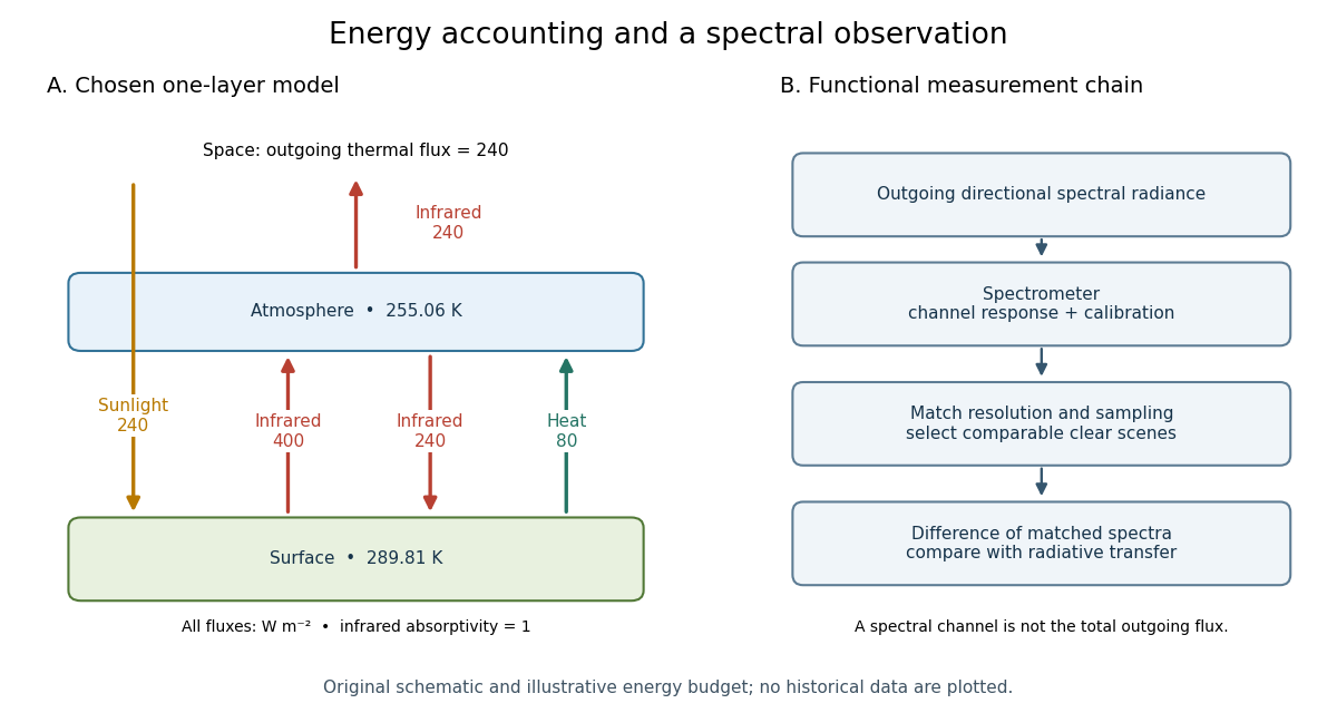
An original two-temperature calculation exposes the bookkeeping. Let an opaque surface absorb solar irradiance $Q$ and emit blackbody thermal radiation $\sigma T_s^4$. A single isothermal atmospheric layer transmits all sunlight and absorbs a fraction $ϵ$ of surface infrared emission, emitting $ϵ\sigma T_a^4$ both upward and downward. This is a grey thermal-band emissivity, with $0<ϵ\le 1$. Let $H$ be upward nonradiative heat flux, and let $C_s,C_a>0$ be heat capacities per unit area. Then conservation of energy givesThe two equations sum toHere $L$ is outgoing longwave radiation. Both $H$ and downward atmospheric emission cancel internally: they redistribute energy without creating it. The factor two in atmospheric emission counts two faces. Dropping the downward face would spoil the surface budget. Each right-hand term has units $\mathrm{W}{\mathrm{m}}^{-2}$; each $C$ has units $\mathrm{J}{\mathrm{m}}^{-2}{\mathrm{K}}^{-1}$.

Choose $Q=240\mathrm{W}{\mathrm{m}}^{-2}$, $H=80\mathrm{W}{\mathrm{m}}^{-2}$ and $ϵ=1$. At equilibrium, $L=\sigma T_a^4=240\mathrm{W}{\mathrm{m}}^{-2}$ and $\sigma T_s^4=400\mathrm{W}{\mathrm{m}}^{-2}$, giving $T_a\simeq 255.06\mathrm{K}$ and $T_s\simeq 289.81\mathrm{K}$. Direct substitution gives surface balance $240+240-400-80=0$ and atmospheric balance $400-480+80=0$. These deliberately chosen fluxes illustrate the model; they are not an observed global budget or a reconstruction of the 1967 calculation. Prescribing $H$ illustrates heat transfer accounting but does not close a realistic convection law.

For fixed $Q,H,ϵ$, the positive-temperature equilibrium is locally stable. Put $a=4\sigma T_s^3>0$ and $b=4ϵ\sigma T_a^3>0$. The Jacobian matrix of the temperature equations has trace $-a/C_s-2b/C_a<0$ and determinant $ab(2-ϵ)/(C_s{C}_a)>0$. Thus both eigenvalues have negative real part. Temperature-dependent climate feedbacks alter this test. A single grey layer also omits the optical spectrum, cloud structure and the independent thermal behavior of the troposphere and stratosphere.

Convective adjustment replaces an excessively steep vertical temperature gradient by an allowed profile while respecting the selected energy budget. It is a closure for unresolved convection, not a direct simulation of individual rising parcels. A prescribed critical atmospheric lapse rate is a modeling assumption; it need not equal the dry adiabatic lapse rate.

For an original dry two-slab example, take fixed equal heat capacities and slab centers separated by $\Delta z=2\mathrm{km}$. Initially $T_1=300\mathrm{K}$ below and $T_2=280\mathrm{K}$ above. Stipulate a permitted atmospheric lapse rate ${\Gamma }_c=6\mathrm{K}\mathrm{k}{\mathrm{m}}^{-1}$. The initial difference $20\mathrm{K}$ exceeds the allowed $12\mathrm{K}$. Conservation of the sum of the two sensible energies requires $T_1^{\prime }+T_2^{\prime }=580\mathrm{K}$, while the adjusted gradient requires $T_1^{\prime }-T_2^{\prime }=12\mathrm{K}$. Hence $T_1^{\prime }=296\mathrm{K}$ and $T_2^{\prime }=284\mathrm{K}$. Heat removed below equals heat added above. Simply holding the lower slab fixed and raising the upper slab to $288\mathrm{K}$ would introduce external energy.

For unequal constant heat capacities $C_1,C_2$, the same two constraints instead giveApply this adjustment only when the original gradient exceeds the threshold. A moist adjustment also has to account for latent heat and changing composition; conservation of this dry sensible-energy expression alone is then insufficient.

The Hasselmann stochastic climate model represents slowly responding climate variables driven by fast weather fluctuations as well as external forcing. Klaus Hasselmann's 1976 paper separates fast and slow variables, retains fluctuations lost by simple averaging, and explains why stabilizing climate feedbacks are needed to prevent indefinitely growing variability. Its general framework is broader than a single-temperature equation.^[ref]

Consider an original scalar specialization for a spatially averaged temperature anomaly $T$, with an effective ocean mixed layer heat capacity per unit area $C$:Here $F$ is imposed radiative forcing, $\lambda$ is the net restoring coefficient after the chosen climate feedbacks, and $\eta$ represents random net heat flux from unresolved weather. The anomaly energy per unit area is $CT$, so its tendency equals the net input. The weather term represents exchange with omitted degrees of freedom; it does not assert that an isolated ocean creates energy. $F$ and $\eta$ have units $\mathrm{W}{\mathrm{m}}^{-2}$, and $\lambda$ has units $\mathrm{W}{\mathrm{m}}^{-2}{\mathrm{K}}^{-1}$.

First set $\eta =0$, start from $T(0)=0$, and switch to constant $F_0>0$. The integrating factor $e^{\lambda t/C}$ givesFor $C=2.0\times 10^8\mathrm{J}{\mathrm{m}}^{-2}{\mathrm{K}}^{-1}$, $\lambda =2.0\mathrm{W}{\mathrm{m}}^{-2}{\mathrm{K}}^{-1}$ and $F_0=4.0\mathrm{W}{\mathrm{m}}^{-2}$, the relaxation time is $10^8\mathrm{s}$, about $3.17$ years using 365.25 days per year. At $t=\tau$, $T=2(1-e^{-1})\mathrm{K}\simeq 1.264\mathrm{K}$, with eventual warming $2\mathrm{K}$. Doubling $C$ doubles the response time but leaves this equilibrium unchanged. This separates thermal inertia from climate sensitivity.

Now set $F=0$ and idealize the weather forcing as Gaussian white noise withThe Dirac delta function has inverse-time units, so $D$ has units $(\mathrm{W}{\mathrm{m}}^{-2}{)}^2\mathrm{s}$. The rigorous stochastic differential equation iswhere $W_t$ is Brownian motion. This is an Ornstein-Uhlenbeck process. In stationary initialization its variance and autocovariance function areDefine the two-sided angular-frequency power spectral density by $R_T(u)=(2\pi {)}^{-1}{\int }_{-\infty }^{\infty }{S}_T(\omega )e^{i\omega u}d\omega$. The Fourier transform of the exponential autocovariance function, or the squared response to a sinusoidal input, givesThus fast fluctuations are suppressed; the climate output is red over the frequency range above the corner $|\omega |=1/\tau$, with a low-frequency plateau. This is a colored noise spectrum without a periodic driver. The corner is $f_c=1/(2\pi \tau )$ in cycles per second, not $1/\tau$. The continuous white input is only an approximation on times longer than weather's correlation time.

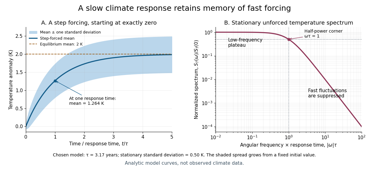
For the same $C,\lambda$ and $D=10^8(\mathrm{W}{\mathrm{m}}^{-2}{)}^2\mathrm{s}$, $v_{\infty }=0.25{\mathrm{K}}^2$ and the stationary standard deviation is $0.50\mathrm{K}$. From fixed $T(0)=0$, the variance grows as $v_{\infty }(1-e^{-2t/\tau })$, even when the forced expected value is predictable. Integrating $S_T/(2\pi )$ over all angular frequencies returns $D/(C\lambda )$, checking the normalization independently. If $\lambda =0$ the unforced variance instead grows as $2Dt/C^2$; if $\lambda <0$, deviations amplify. Neither case has the stationary spectrum above.

A red spectrum alone cannot establish attribution of recent climate change: internal variability, changing forcing and measurement effects must be distinguished. This scalar model supplies a calculable baseline for variability and persistence, not a universal spectrum for all climate timescales or a full attribution analysis.

A satellite test of greenhouse spectral change compares outgoing radiance with radiative transfer predictions. The 2001 study compared IRIS on Nimbus 4 (1970) and IMG on ADEOS (1997). Matching April–June ocean regions, masking land, screening clouds and correcting resolution and wavenumber controlled comparability. Spectral radiance became brightness temperature readouts. Regional comparisons and independent calculations tested interpretation. Carbon dioxide and methane features supported changed absorption; residual clouds, calibration and interannual variability limited background inference.^[ref]

This observational comparison tests radiative transfer; it does not by itself measure equilibrium climate sensitivity or validate a complete climate model.

To understand the readout, write an instrument's spectral channel schematically asHere $I$ is spectral radiance in the viewing direction $\hat{\mathbf{n}}$, $K_j$ is a normalized channel response, $b_j$ is calibration offset and $e_j$ is random error. Subtracting two channel readings isolates an atmospheric difference only after their response functions and sampling are comparable. Matching kernels reduces a false difference caused merely by observing a narrow spectral line at different resolutions; it cannot remove every calibration offset.

Outgoing longwave radiation in an energy budget also integrates radiance over upward directions and over the thermal spectrum, with the appropriate projected-angle factor. A brightness temperature converts one spectral radiance to the equivalent blackbody value through Planck's law; it is not automatically surface temperature. This explains why a spectral difference, a broadband radiative flux difference and surface warming are related observables with different units and different inferences.